

01The idea
A STAC catalog (SpatioTemporal Asset Catalog) describes each scene as a GeoJSON feature: its outline, its date, its cloud cover, and links to its files, one per band. Those files are cloud-optimized GeoTIFFs: tiled, with overviews, so a program can read just the part of a scene it needs. Janus asks the catalog for the scenes, groups them by day, and makes each day one image of the area on one grid. Nothing is downloaded until it is drawn, and then only the blocks and the overview level on screen.
- Collection
- A product of the catalog: Sentinel-2 L2A, Landsat Collection 2 Level-2, a data cube.
- Item (scene)
- One acquisition of one tile of a collection:
S2B_MSIL2A_20190610T142759_..._T20LNP. - Asset
- A file of an item: a band (
B04,red), the quality band, a thumbnail. Janus uses the single-band GeoTIFFs. - STAC API
- The catalog's search: a
POST /searchwith the collection, the area, the dates and a limit, answered page by page.
02The catalogs
File → Search STAC catalog... opens a window with three catalogs ready, each with the collections a series of reflectances needs, and any other STAC API by its URL:
| Catalog | Collections | Access |
|---|---|---|
| Earth Search (Element 84, AWS) | Sentinel-2 Collection 1 L2A, 10–60 m, every 5 days, 2015 on | public, no account |
| Planetary Computer (Microsoft) | Sentinel-2 L2A; Landsat Collection 2 Level-2 (Landsat 4 to 9, 30 m, 1982 on); Sentinel-1 RTC (radar, VV and VH, 10 m, 2014 on) | short-lived tokens (SAS) that Janus asks for and renews, no account |
| Brazil Data Cube (INPE) | 16-day cubes of Sentinel-2 (10 m), Landsat (30 m) and CBERS-4 WFI (64 m) on a regular grid | public, no account |
| Another STAC API | any, from List all (its /collections) | public files |
List all also lists the other collections of the three catalogs (Harmonized Landsat Sentinel, MODIS...). Janus finds their bands from the items: their names, their wavelengths (eo:bands), their scale, offset and nodata (raster:bands).
03Searching
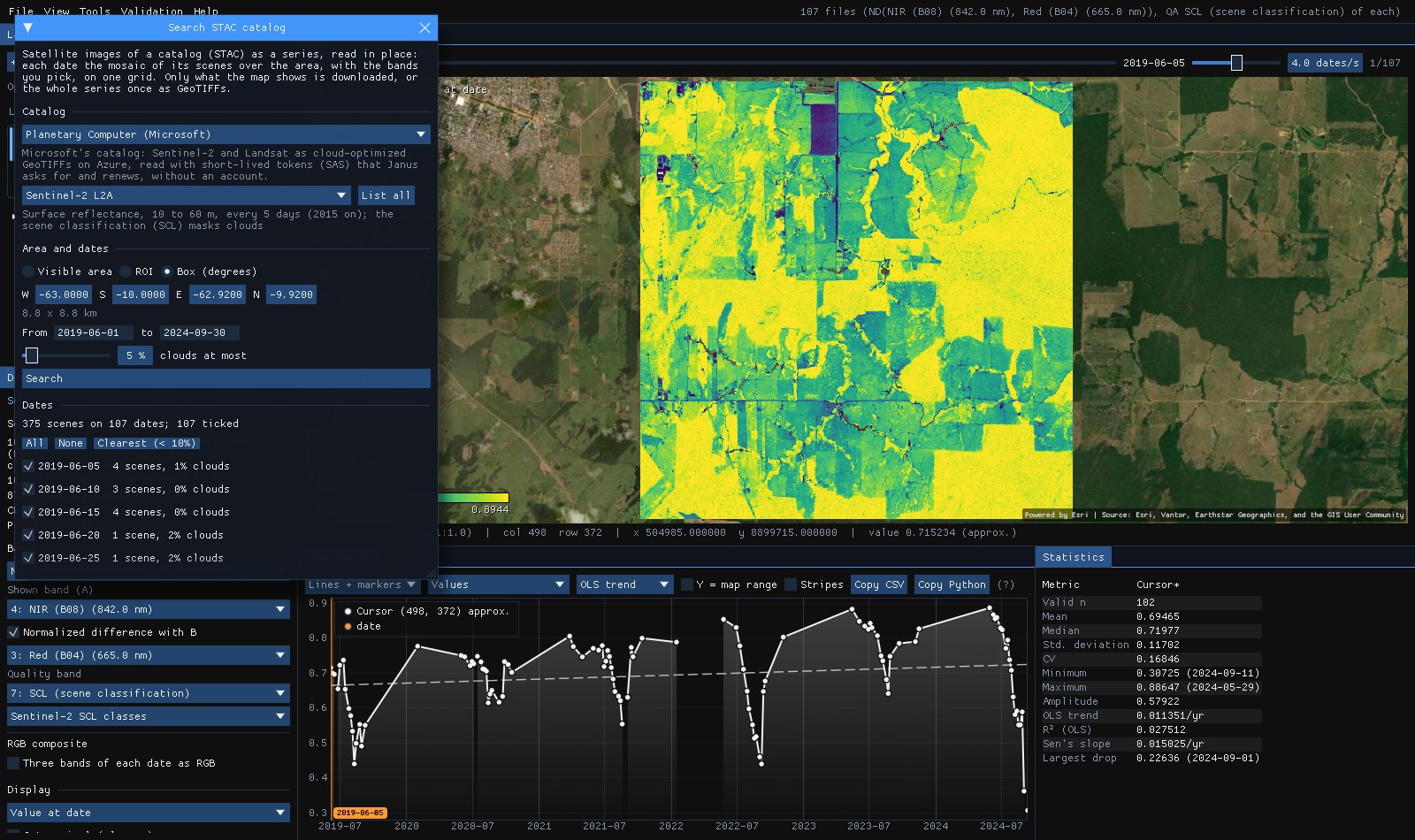
The example: Planetary Computer's Sentinel-2 L2A over a square of central Rondônia, Brazil, 8.8 km a side (63.00° to 62.92° W, 10.00° to 9.92° S), from June 2019 to September 2024, scenes with 5% of clouds at most.
- Area
- Visible area (the map's extent), the ROI, or a Box in degrees (west, south, east, north). With no layer open, the box.
- From, to
- The dates, inclusive (YYYY-MM-DD). The last 365 days at first.
- Clouds at most
- The scenes' cloud cover (
eo:cloud_cover) as the catalog gives it: of the whole scene, not of the area. 100 keeps them all.
Search found 375 scenes on 107 dates. The square sits where four Sentinel-2 tiles meet, so a date has up to four scenes. Each date is listed with its scenes and their mean cloud cover, all ticked: untick the ones you do not want, or Clearest (< 10%) keeps the dates under 10%.
04Bands and cells
Under the dates, the collection's bands, in the order of their wavelengths. Blue, green, red, NIR, the two SWIR and the quality band come ticked: enough for every index Janus computes, the RGB composites and the cloud mask, and a third of what all the bands would weigh.
- Quality band
- Sentinel-2's scene classification (
SCL): classes 4, 5 and 6 (vegetation, bare soil, water) are kept, clouds, their shadows, cirrus and snow are masked. Landsat'sQA_PIXEL: its fill, cloud, dilated cloud, cloud shadow and snow bits. Janus picks it as the layer's quality band. - Cells
- Finest of the bands (10 m for Sentinel-2), or 20 to 250 m: coarser cells average the reflectances (the quality band takes the nearest code), for large areas. The window gives the size of the series: here 877 × 886 cells of 10 m, 107 dates × 7 bands.
Sentinel-2's offset
Since processing baseline 04.00 (January 2022), ESA's L2A reflectances carry an offset of −0.1: a value of 1000 is a reflectance of 0. Planetary Computer's items do not say so; Janus reads each scene's baseline and gives its bands the scale and offset that make every date comparable, so the NDVI does not jump in 2022.
05Open as a layer
Open as a layer runs as a task (Tools → Tasks): it writes one VRT per date under %LOCALAPPDATA%\Janus\results\stac, each a mosaic of that day's scenes pointing at the catalog's files, and opens the folder as a layer. With red and NIR among the bands the layer opens on the NDVI, with the quality band masking clouds, like any Landsat or Sentinel series on disk.
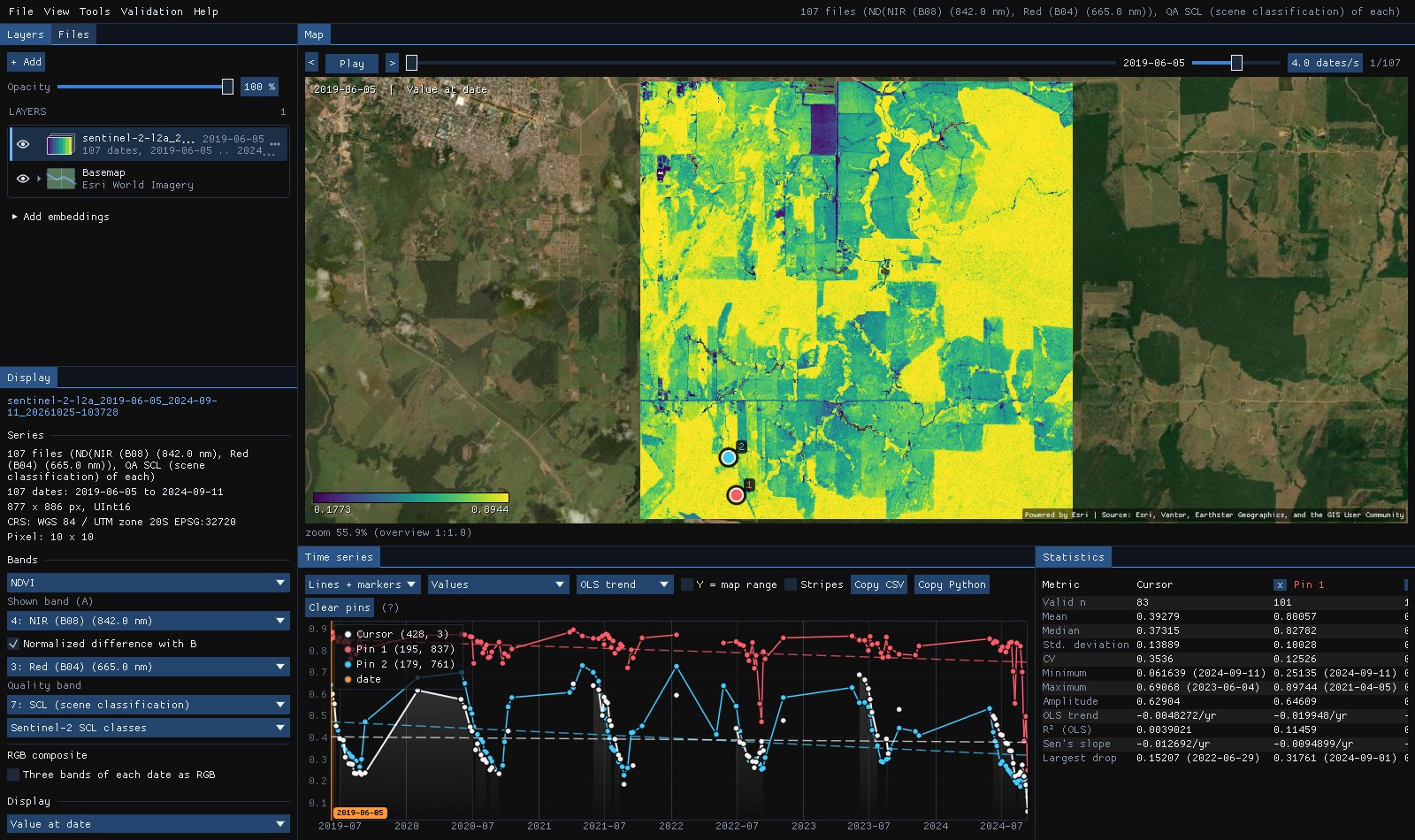
Pin 1 sits in a forest: its NDVI stays around 0.8 (mean 0.80 over 101 dates) and only falls, to 0.25, at the end of the 2024 dry season, its largest drop. Pin 2 is a pasture: green in the wet months, down to 0.25 every dry season. Six of pin 1's 107 dates are missing: the scene classification called that pixel cloud, shadow or cirrus on them, and the mask left them out, though the scenes had 5% of clouds at most.
The map's overview of the 107 dates was read in 98 s: every date opens its scenes over the network and reads one of their overview levels. It is then cached on disk like any series: opening the folder again, the overview took 0.1 s. A pixel's series reads every date from the catalog's files, a few round trips each, so Janus reads twelve dates at once: the two pins' 107 dates came in under a minute (one date at a time, they took nine). Zoomed in, the map reads the blocks on screen at full resolution, as for any cloud-optimized GeoTIFF.
Read in place: online
The layer reads the catalog's files as you zoom in and look at pixels, so it needs the connection while you work. Planetary Computer's files are read with tokens that expire within the hour: Janus renews them in the background, and asks for new ones when the folder is opened again another day. For offline work, download the series (section 07) or a composite of it (section 08).
06One grid for every date
Scenes come in tiles, each in its own projection, and bands come at 10, 20 or 60 m. A series needs one grid. Janus makes it from the scenes found:
- Projection
- The one most scenes have: here UTM zone 20 S. The area's corners and edges are projected to it.
- Cells
- The finest band's, aligned on the scenes' own pixels, so a 10 m band is read without resampling.
- Mosaic
- A date's scenes are drawn clearest on top, each clipped to its pixels in the area. The quality band of a 20 m scene is taken at the nearest cell; reflectances at coarser cells are averaged.
- Another UTM zone
- A scene in another projection (where the area crosses a zone boundary, as along 60° W) is warped onto the grid by GDAL's warped VRT, still read in place.
Brazil Data Cube's cubes are already on a regular grid of their own (BDC's Albers), and give one image every 16 days: the best observation of each pixel. Their items have no projection metadata; Janus reads it from one file of each tile.
07Download as GeoTIFFs
Download as GeoTIFFs makes the same series and reads it once, writing one cloud-optimized GeoTIFF per date (DEFLATE, the bands of the date, their wavelengths, scales and nodata kept) into a folder under results\stac, then opens it. Its progress is in Tools → Tasks, where it can be cancelled; a date is written to a .part file first, so a folder never holds a half-written date.
The window gives the size before you start: here 877 × 886 cells, 107 dates × 7 bands, about 1.2 GB uncompressed, less on disk. For a larger area or a longer series, coarser Cells or fewer bands make it lighter; the Clearest dates alone too.
08Download a composite
Often one image of a season is what is wanted, not the series: a map of the dry season, a mosaic without clouds to classify. Composite, under the bands, makes it from the dates ticked, each pixel from the date that suits it best, and downloads only that: Download the composite writes a cloud-optimized GeoTIFF (or one a year of the dates of each year, for the same season of several years) and opens it as a layer.
- Best available pixel
- Each pixel's clear observation of the highest score (after Griffiths et al. 2013 and White et al. 2014), every band from that date. The score adds four things, weighted 0.3, 0.5, 0.1 and 0.1: how near its day of the year is to the target day (a Gaussian of ± 30 days around it; the middle of the dates unless typed as MM-DD), how far the pixel is from the nearest cloud or shadow of its date (0 at 30 m or nearer, 1 at 1500 m or farther, 1 on a date without clouds), its sensor (Landsat 7 after its scan line corrector failed in 2003 scores 0.5) and its scene's cloud cover. The same as zeit's
build_annual_composites(method="bap"). - Greenest
- The clear observation of the highest NDVI, Earth Engine's
qualityMosaic: the peak of the season. - Medoid, median
- The clear observation nearest the bands' medians (a real date, every band from it), or each band's median.
- Info
- A second GeoTIFF in the composite's
infofolder: each pixel's year and day of the year, its score and its number of clear observations.
The composite opens as a layer of its six bands, their wavelengths kept, so in true colour; the Display panel's indices and composites work on it as on any spectrum.
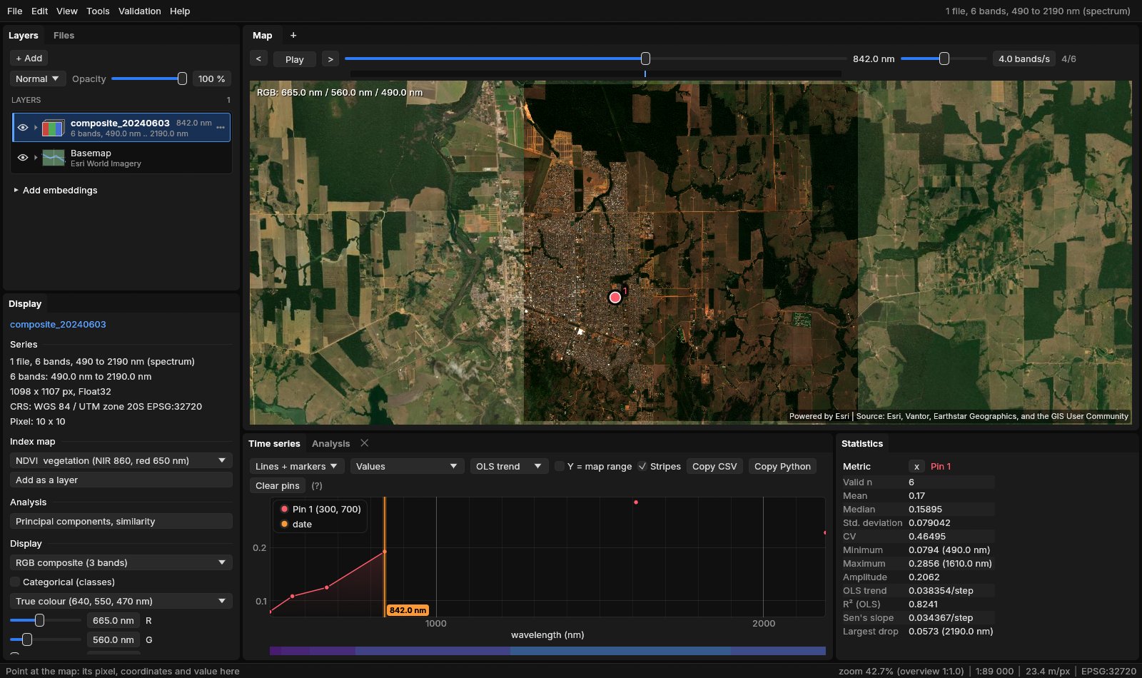
The best available pixel needs only the quality band to choose: Janus reads it for every date first, block by block (1024 pixels with the cloud distance around them, so the clouds of the neighbouring blocks count), chooses each pixel's date, then reads the bands of the dates that won in the block, over the box of their winners. Where a winner has no value in a band (the edge of a scene) the pixel takes its next best date. The rest of the series is never downloaded. The greenest reads the red, NIR and quality bands of every date; the medoid and the median, every band of every date: what downloading the series would.
On Earth Search's Sentinel-2 C1 L2A over a square of 11 km of Rondônia (63.05° to 62.95° W, 9.95° to 9.85° S), June to September 2024 with 70% of clouds at most: 46 scenes on 24 dates, 1098 × 1107 cells of 10 m, six bands and SCL. Four threads, GDAL's caches emptied before each composite, the bytes from GDAL's network statistics:
| Composite | Time | Downloaded | Pixels read |
|---|---|---|---|
| Medoid (every date's bands) | 541 s | 1992 MB | 204 million (all) |
| Greenest | 560 s | 1804 MB | 189 million (93%) |
| Best available pixel | 241 s | 572 MB | 92 million (45%) |
The best available pixel downloaded 29% of what the medoid did, in 45% of the time. Its target day was the 196th (14 July): 99.4% of its pixels came from 13 July, a clear date, and the rest, near that date's few clouds, from 13 other dates. A pixel had 21 clear observations in the median, 7 at the fewest.
09Footprints
Footprints as a vector layer adds the scenes found as polygons, with their id, date, cloud cover and tile in the attribute table: where each tile lies, and which dates cover only part of the area.
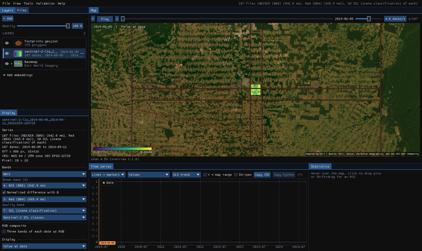
The strips are the tiles' overlaps (Sentinel-2's 110 km tiles overlap by 10 km): the square sits inside four of them, which is why a date has up to four scenes, the same pixels in several. Where an orbit's swath ends, a scene covers part of its tile only (the diagonal): on such dates the mosaic takes the rest from the other scenes of the day, or leaves it empty.
10Sentinel-1: radar through the clouds
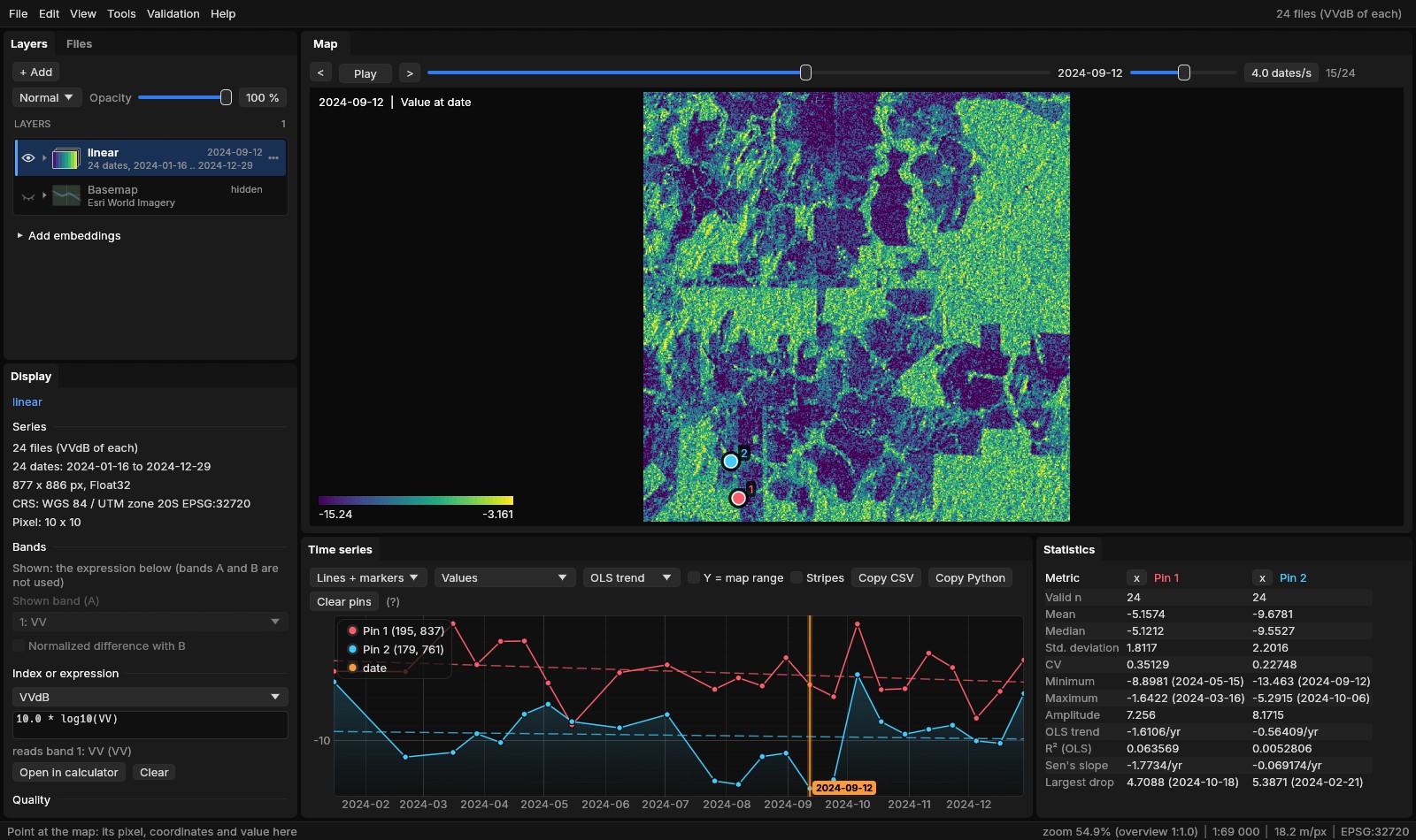
In Rondônia the clear optical scenes thin out from October to April: with 5% of clouds at most, the series above has 107 dates in five years. Sentinel-1's radar sees through the clouds, every 12 days whatever the weather. Planetary Computer's Sentinel-1 RTC collection gives its backscatter in VV and VH as gamma0 already corrected for the terrain, at 10 m, as cloud-optimized GeoTIFFs read with the same tokens.
The same square, all of 2024: 24 scenes, every one of the descending pass of relative orbit 83 (09:49 UTC, about 05:49 local time).
- Pass
- Above the dates, Pass lists the satellite's passes over the area: its direction (ascending or descending) and its relative orbit, with their scenes. The pass with the most scenes is kept at first. Scenes of two passes see the ground from opposite sides and other angles: mixed in one series they make false steps every few days. All passes (mixed) is there when you want them anyway.
- Clouds
- The cloud slider and Clearest are gone: radar scenes have no cloud cover, and no quality band.
- Bands
- VV and VH, both ticked. Their values are linear powers (0.01 to 0.3 over land); the layer opens in decibels, the VVdB index (
10 * log10(VV)). The Display panel's index list has VHdB, VHVVdB (the ratio VH/VV in dB) and the library's radar indices (the dual-polarized RVI, the polarization ratios, differences and sums).
Read whole as VV in dB, the 24 dates of 877 × 886 cells took 3.9 s, every value equal to stackstac with numpy's 10 * log10 on the same items and grid, and to rasterio on a scene alone.
Speckle
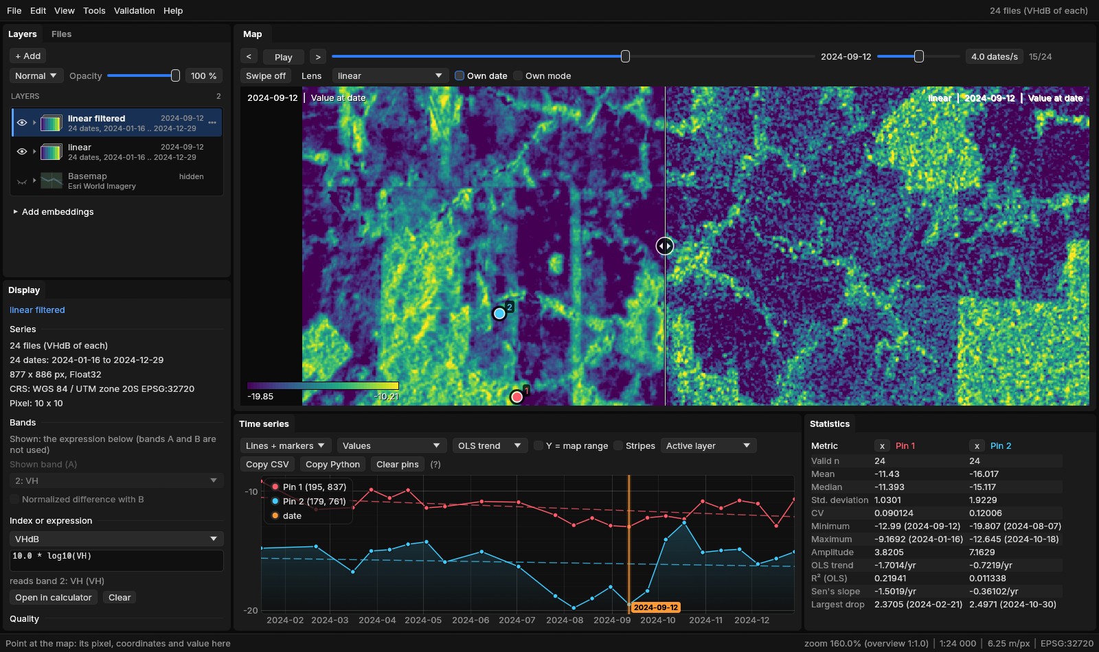
Radar images are grainy: each cell sums the echoes of many scatterers, which add up or cancel at random. This speckle is not noise to be fixed but part of the signal; it is averaged away, over neighbouring cells or over dates. Tools → Data preparation → Speckle filter... writes a filtered copy of the series:
- Quegan (multitemporal)
- Each date's window mean times the mean, over all the dates, of each date's value divided by its own window mean (Quegan & Yu 2001). The speckle is averaged through time, so a date keeps its own changes and the cells keep more detail than a window alone would leave.
- Lee (spatial)
- Each date alone: the window's mean, plus the cell's departure from it in proportion to how much more the window varies than speckle of that many looks would (Lee 1980; Sentinel-1's IW scenes have 4.4). Smooth fields are averaged, edges kept.
Both work on the linear values, whatever the layer shows, and the filtered series opens in dB like the one filtered. Over the square, a 7 × 7 window of Quegan's filter took 1.7 s for the 24 dates of both bands, written as COGs: the same values as the formulas through scipy.ndimage (to 1.3e-7), which took 2.1 s for the arithmetic alone.
The dry season
The radar follows the season where the optical scenes stop. On the five largest patches whose VH fell by more than 3 dB between the year's first six dates and its last six (10 to 12 ha each, around 62.966° W, 9.982° S), VH holds at −12 to −13.5 dB from January to May, falls through June, July and August, and stays near −20 dB from mid-August to the end of September; with the rains it comes back to between −12 and −18 dB from October, rising and falling with wet and dry spells. They are pastures drying out: in the Sentinel-2 series above their NDVI fell from about 0.4 at the end of May 2024 to 0.09 on 11 September, lower than in any dry season since 2019 (lows of 0.16 to 0.26), and rose again with every rainy season. The forest of pin 1, whose NDVI fell to 0.25 at the end of that dry season, keeps its VH between −9 and −13 dB all year (after Quegan's filter): the radar sees a canopy that dried, not one that fell.
One pass, one series
CUSUM, BEAST and the trend tools work on the dB series as they are. The tools that want a fixed step (BFAST, BFAST Monitor) want Tools → Data preparation → Regularize series... first: the 12 days of one pass become 12 or 16 days exactly.
11What next
- Detect change on it: a series of every date suits CCDC, S-CCD and EWMACD; a regular one (Brazil Data Cube's 16 days) BFAST and BEAST.
- Classify it: the Deep learning guide trains TempCNN or L-TAE on samples over the series.
- Its embeddings: AlphaEarth or TESSERA of the same area, from the Layers panel (Embeddings guide).
- Script it: the VRTs open in GDAL, QGIS or Python (
rasterio.open) like the files they point at; Planetary Computer's need a signed URL there (planetary_computer.sign).
12References
- STAC: the SpatioTemporal Asset Catalog specification and its API, stacspec.org.
- Earth Search by Element 84, element84.com/earth-search; Sentinel-2 Collection 1 L2A, Copernicus Sentinel data (ESA).
- Microsoft Planetary Computer, planetarycomputer.microsoft.com.
- Ferreira, K. R., et al. (2020). Earth observation data cubes for Brazil: Requirements, methodology and products. Remote Sensing, 12(24), 4033.
- ESA (2022). Sentinel-2: new processing baseline 04.00 and the radiometric offset of the L1C and L2A products.
- U.S. Geological Survey. Landsat Collection 2 Level-2 Science Products.
- Sentinel-1 Radiometrically Terrain Corrected (RTC), Planetary Computer, from Copernicus Sentinel-1 data (ESA), processed by Catalyst.
- Griffiths, P., van der Linden, S., Kuemmerle, T., & Hostert, P. (2013). A pixel-based Landsat compositing algorithm for large area land cover mapping. IEEE Journal of Selected Topics in Applied Earth Observations and Remote Sensing, 6(5), 2088–2101.
- White, J. C., Wulder, M. A., Hobart, G. W., Luther, J. E., Hermosilla, T., Griffiths, P., et al. (2014). Pixel-based image compositing for large-area dense time series applications and science. Canadian Journal of Remote Sensing, 40(3), 192–212.
- Quegan, S., & Yu, J. J. (2001). Filtering of multichannel SAR images. IEEE Transactions on Geoscience and Remote Sensing, 39(11), 2373–2379.
- Lee, J.-S. (1980). Digital image enhancement and noise filtering by use of local statistics. IEEE Transactions on Pattern Analysis and Machine Intelligence, PAMI-2(2), 165–168.