Open
Any stack of rasters
A folder (one file per date), a multiband file (one band per date), a list of files or a wildcard. Dates are read from file names or band descriptions.
YYYY-MM-DD · YYYYMMDD · YYYY_MM · YYYY · A2001001


Raster time series analysis · Windows · macOS · Linux
Explore satellite imagery pixel by pixel, find where, when and by how much the land changed, and measure how accurate your maps are.
jn D:\data\ndvi_annual\jn ~/data/landsat_stack.tifjn "S2_*_NDVI.tif" --band 1After installing, jn opens the window and gives the prompt back right away.
How it works
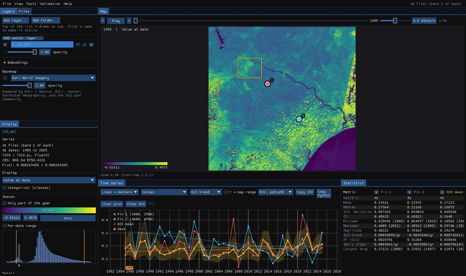
Each date is one layer of the cube. Janus keeps a reduced copy of all of them in GPU memory, computes the per-pixel statistics in a shader and, while the mouse rests, reads the full-resolution series of that pixel from disk in the background.
Features
Open
A folder (one file per date), a multiband file (one band per date), a list of files or a wildcard. Dates are read from file names or band descriptions.
YYYY-MM-DD · YYYYMMDD · YYYY_MM · YYYY · A2001001
Catalogs
Search Earth Search, Planetary Computer, the Brazil Data Cube or any STAC API for an area, two dates and a cloud cover, and open the scenes as a series read in place: a mosaic per date on one grid, clouds masked. Or download them as GeoTIFFs, or only a composite of them: the best available pixel, which never downloads most of the series. Sentinel-1's radar too, one pass at a time, in dB. Step-by-step guide.
Sentinel-2 · Landsat · Sentinel-1 RTC · BDC cubes · SCL · QA_PIXEL
Calculator
The 275 Awesome Spectral Indices on any series, or an expression of its bands; Tools → Raster calculator combines the open layers by short names, reduces a series over time, by year or month, over calendar windows and windows in days, with lags, anomalies and events, and reclassifies by rules, computed as the map reads it. Step-by-step guide.
EVI · max(ndvi) · ndvi[2019-06 .. 2019-09] · mean(ndvi, 90d) · anomaly(...) · first(...)
Map
Value at date, anomaly, mean, standard deviation, linear trend, minimum, maximum, amplitude, trend R² and a multitemporal RGB. Changing the date, colormap or stretch is instant.
13 map modes · animation player
Series
An approximate series appears as soon as you hover and the exact one once the mouse rests. Click to drop pins; Shift+drag for a region with its mean and p10–p90 band.
OLS and Sen trend · anomaly · z-score
Classes
Land cover and classification stacks are detected from colour tables or category names. The chart shows the class sequence and the table reports the last change.
e.g. 2006: Forest → Pasture
Bands
Show any band of a Landsat or Sentinel stack, or a normalized difference of two, and hide cloudy observations with a quality band.
NDVI · NDMI · NBR · Fmask · QA_PIXEL
Layers
Open several series as layers placed by their georeferencing, and show them in map panels that pan and zoom together, each at its own date and mode. Drag any panel to a second monitor.
Ctrl+T / Ctrl+W · 2005 next to 2020 · NDVI next to NBR
Detail
Past the overview resolution, tiles of the visible area are read in the background and cached on the GPU. The overview is cached on disk date by date, so reopening takes a fraction of a second and closing during the first open loses nothing.
COG-friendly · HDD-aware reader
Change
Map the difference from a reference date, or from the previous one, on a diverging scale. Or map when the largest drop happened and how deep it was, computed for every pixel on the GPU.
Δ to a date or t−1 · drop date · drop magnitude
Compare
Drag a divider across the map to compare it with another layer, or with the same layer at another date or in another mode.
S to toggle · 1985 | 2025 · NDVI | NBR
Space-time
Draw a line on the map and see distance against time in one image: deforestation fronts and regrowth appear as shapes. Hover marks the place on the map, a click goes to that date.
Ctrl+drag · values or anomalies · CSV
Visualize
A map of the places whose series is like this one's, by values or by shape, following the cursor; a place's cycles by wavelet; every band over time; and every pixel's behaviour in a UMAP plane linked to the map. The Analysis panel sits next to the time series and shows only the views the data allow. Step-by-step guide.
Similarity · Cycles · Bands · Atlas
Export
Save the map as a PNG for figures, at up to 4× the screen resolution, with legend and date. Save the values or the rendered view as a georeferenced GeoTIFF for QGIS, and the series as CSV.
PNG · GeoTIFF · Zeit results · CSV
Analysis
Fit LandTrendr, BFAST, CCDC and other Zeit tools live on the cursor and pins, or run them on the image, with the results added as map layers.
16 tools · no Python to install
Validation
Stratify any map, draw a sample, interpret it blind with chips of every date, and get the accuracy and error-adjusted areas with confidence intervals (Olofsson et al. 2014). Step-by-step guide.
strata · blind labels · kappa · HTML report
Deep learning
Train TempCNN, L-TAE or U-TAE on samples you already have in Janus (a vector layer's class column, pins, an interpretation, a validation project), or classify on Presto's pretrained encodings, on the GPU and without Python. A class map, its probability and its uncertainty come back as layers, and the model's area of applicability: where the image is unlike its samples. Step-by-step guide.
TempCNN · L-TAE · U-TAE · Presto · area of applicability · .janusmodel
Objects
SNIC cuts the image into segments whose pixels share a history, with each segment's mean series as a layer and their polygons as a vector layer, to interpret, run the tools on or sample by object. Step-by-step guide.
SNIC · mean series · polygons
Objects
WRI's Trazo and Fields of The World's networks draw every field's boundary on two composites of a Sentinel-2 season, on the GPU and without Python, with WRI's published accuracy; a watershed turns them into parcels that touch. Draw a few fields of your own and fine-tune the network on them. Step-by-step guide.
Trazo · FTW · watershed parcels · fine-tuning · .janusfields
Workspace
Ctrl+K finds any menu, tool, index, layer or panel by name. A status bar gives the pixel, coordinates, value, CRS and scale, and tells you when a task ends. Layers blend and group, and copy their style; Go to a place, save views, a minimap and a lens. Step-by-step guide.
Ctrl+K · Ctrl+G · blend modes · groups · saved styles · minimap · lens
Projects
A project keeps the layers, styles, dates, views, pins and ROI, and the last session comes back when you open Janus. Ctrl+Z undoes a change to the layers. Every result records how it was made (tool, parameters, inputs, versions), to run again or copy as Python, and a tool's preview on the ROI comes before the whole scene.
Ctrl+S · Ctrl+Z · provenance · Copy Python · preview
Series
Build a series from loose files (dates from their names, bands and tiles told apart), put an irregular one at a fixed step (median, medoid or clearest date, gaps filled), and save any series as a multiband COG, a NetCDF or a Zarr with its time axis, ready for xarray. Step-by-step guide.
VRT · COG · NetCDF CF · Zarr · 16 days · monthly · Whittaker
Maps to numbers
Reproject, resample or clip with gdalwarp's own code; polygonize a map with each patch's geodesic area; the true area of every class at every date; rasterize polygons on the series' grid; statistics and class areas of every polygon through time. Step-by-step guide.
GeoPackage · ha by class and year · transitions · zonal CSV
Radar
Sentinel-1 RTC from Planetary Computer, one orbit pass at a time, shown in dB with VH/VV and the radar indices; Quegan's multitemporal or Lee's speckle filter makes a smoother series that keeps each date's changes. Step-by-step guide.
VV · VH · dB · Quegan · Lee
Change detection
The Zeit algorithms are fitted live on the cursor, pins and region, or run on the whole image, the visible area or a region, with the results added as map layers. Zeit's methods are part of Janus, so there is nothing else to install, and a fit on the chart takes under a millisecond.
Year of detection, magnitude, duration and rate of the chosen loss or gain event.
annual seriesAfter LandTrendr's loss: years to recovery (Y2R), R80P, RRI and the absolute and year-on-year recovery.
annual seriesEvery observation against its training years through EWMA control charts: when it was disturbed, how far, when it recovered or gained, its state now.
any dates, ≥ 2 per yearWhere values cluster high or low and how that changed: the Getis-Ord Gi* of every date and its trend, as ESRI's patterns (new, intensifying, persistent, sporadic... hot and cold spots).
≥ 3 datesSignificant Sen's slope, p-value and trend class, with Hamed-Rao, Yue-Wang and seasonal variants.
any seriesThe trend's t-test with autocorrelated errors (remotePARTS), and the regional Trend test by PARTS.
any seriesTrend and season break counts, date and magnitude of the largest break.
≥ 2 dates per yearBreak count, date and magnitude of the largest break, first break date.
≥ 2 dates per yearFirst break in the monitoring period, its magnitude, break yes or no.
≥ 2 dates per yearTrend and season averaged over thousands of models: the probability of a changepoint at each date, the most probable one with its jump, the mean number of changepoints.
any series, ≥ 12 datesStart, peak and end of season, length, amplitude, for a typical year or a chosen one.
≥ 6 dates per yearBreak count, largest break, NDVI change and segments from every reflectance band.
one file per date, multibandCCDC's models carried forward by a Kalman filter: the breaks, and the state of every pixel at the last date (stable, change in progress and since when, waiting for a model).
one file per date, multibandForest degradation and deforestation from the NDFI of every observation, as strata and change dates.
one file per date, multibandSpectral unmixing of every date into a new layer of the NDFI, ready for the other tools.
one file per date, multibandThe fraction of each cover (vegetation, soil, water...) whose spectrum you take from pins, at every date or in a hyperspectral scene.
multiband or spectrumThe clouds and shadows the quality band missed, and the series without them as a new layer.
green and SWIR1A class map from patterns you take from pins on places you know.
classificationA classification cleaned: one-year flickers removed, a majority filter and a minimum mapping unit; models' probabilities smoothed as sits does.
classesClusters of alike trajectories, with the typical series of the one under the cursor.
clusteringCompact clusters of the whole series, named by the classes of your samples in them.
clusteringWhere and when several change maps agree: the consensus year and how many back it.
on result mapsWhittaker and Savitzky-Golay, drawn over the series on the chart.
chart onlySegments of alike series, their mean series as a layer and their polygons as a vector layer.
segmentationGuides
Each guide follows one dataset from the first look at its series to the maps a tool makes of it, with screenshots of every step taken by Janus itself.
Forty years of a Rondônia forest frontier as straight segments: the year, magnitude and duration of every clearing, and how long the forest took to recover.
Harmonic models of every band, breaks when the land changes, and a cloud-free image of any date.
CCDC's models carried forward by a Kalman filter: a forest cleared in 2023, and one being cleared now, shown as a change in progress before it is confirmed.
Forest degradation apart from deforestation, from the NDFI of every observation.
Thinning and harvests in pine stands found by EWMA control charts on every date, cloudy ones included: when, how strong, and when they recovered.
Breaks in trend and season of a 16-day EVI series: BFAST, BFAST Lite and BFAST Monitor.
Changepoints with their probability: a clearing BEAST is sure of, a rise it gives 61%, a forest where it claims no change, and maps of how sure it is.
The start, peak, end and length of the growing season of every pixel.
Whether a region, or each land-cover class, is really trending, when a quarter of its pixels say so.
Where forest and cleared land cluster in forty years of Rondônia, and how that changed: new, intensifying, oscillating or historical hot and cold spots.
How much forest, soil and water is in each pixel: every date of a Landsat series and every pixel of an EnMAP scene, from endmembers picked with pins.
Strata, a sample, blind interpretation, accuracy and error-adjusted areas with confidence intervals.
Segments of pixels with the same history, their mean series as a layer and their polygons.
A year of Sorriso as 430 field parcels in three seconds, Trazo's published accuracy matched, and the network fine-tuned on fields you draw.
TempCNN, L-TAE and U-TAE trained on MapBiomas samples: a land cover map with its probability and uncertainty, smoothed, and where the model can be trusted.
A pretrained foundation model's encodings of every pixel: embeddings to explore, and a classifier on them.
EVI and the 275 Awesome Spectral Indices on a Sentinel-2 series, the open layers combined by short names, 107 dates reduced to an image, classes by rules.
An area, two dates, a cloud cover: 375 Sentinel-2 scenes of five dry seasons as a series of 107 dates, read in place from Planetary Computer with the clouds masked; then a year of Sentinel-1 radar over the same square, in dB, a clearing seen through the clouds.
36 loose files built into a series, 107 irregular Sentinel-2 dates put every 16 days with their gaps filled, saved as a NetCDF and a Zarr that xarray reads, and a year of Sentinel-1 through a speckle filter.
34 years of MapBiomas on a Landsat series' grid: the hectares of each class every year, the forest patches of 1985 as polygons, and what became of each one, year by year.
Forest, pasture and water from nine pins in milliseconds, what changed into what since 2017, and the direction of every change.
Every pixel compared with a forest and with a pasture, the forest's yearly cycle by wavelet, its six bands over time and 41 years of Landsat as three behaviours in a UMAP plane.
The status bar and notices, Ctrl+K for any command, Ctrl+G for any coordinate, blend modes, groups and styles, a lens on another date, the provenance and Python of every result, previews, projects and undo.
Install · latest release
Each package carries GDAL and the PROJ and GDAL data; Zeit is part of the program. No Python or conda needed.
Run the installer. It installs per user, without an administrator prompt, and can add jn to PATH, an Open in Janus entry to the right-click menu of folders and .tif files, and a desktop shortcut.
janus-<version>-setup.exe
Open the disk image and drag Janus into Applications. The app is not signed with an Apple Developer ID: the first time, open it with right click → Open. To call it from a terminal, link it once:
ln -s /Applications/Janus.app/Contents/MacOS/janus ~/.local/bin/jnjanus-<version>-macos-arm64.dmg · macOS 15 or later
Extract the archive anywhere and run jn from that folder. It is portable: only glibc, the graphics drivers and X11 or Wayland come from the system. janus.desktop is included for a menu entry.
janus-<version>-linux-x86_64.tar.xz · tested on Ubuntu 24.04
Prefer to build it yourself? Building from source needs Rust and GDAL.
Command line
The command line only opens and shows. Bands, indices, cloud masks and the Zeit tools live in the interface.
# every raster in the folder, 1 file = 1 date
jn D:\data\ndvi_annual\

# 1 multiband file, 1 band = 1 date
jn landsat_stack.tif

# a wildcard pattern, band 1 of each file
jn "S2_*_NDVI.tif" --band 1

# options
--band N        band used when each file is one date
--budget MB     memory for the cube overview (default 1024)
--threads N     background reader threads (HDD = 1)
Questions
No. It is made for time: open a series, move through it, inspect any pixel, detect change with the Zeit tools and validate the maps they make. For editing vectors or laying out maps, keep using your GIS: Janus hands it GeoTIFFs, PNGs, CSVs and GeoPackages.
Anything GDAL reads, as a folder of rasters (one date per file), a multiband file (one date per band), a list of files or a wildcard pattern; also cloud-optimized GeoTIFFs by URL, and the scenes of a STAC catalog (File → Search STAC catalog...). Cloud-optimized GeoTIFFs open fastest the first time.
No. Zeit's methods are compiled into Janus: nothing runs in Python, and nothing starts until you use a tool.
Janus detects spinning disks and reads them with a single sequential reader, which was measured to be four times faster than two. The first open is bound by the disk; after that the cube comes from the overview cache. The cache is written date by date, so if you close Janus halfway, the next open reads only the dates still missing.
Janus is the Roman god of doorways and of time, shown with two faces: one looks at the past and one at what comes next. That is what you do with a pixel's series. Up to version 0.16 the program was called tsv.