LandTrendr · Janus

01The idea

An annual series of a vegetation index is noisy: a dry year, a haze the composite missed, a field ploughed in one year and not the next. LandTrendr (Kennedy et al. 2010) looks for the few vertices, the years where the trajectory changes direction, joined by straight segments, that explain the series best with as few breaks as possible. A segment that goes down is a loss (a clearing, a fire, a harvest); one that goes up is a gain (regrowth, a plantation). From the segments, Janus maps one event per pixel: its year of detection, magnitude, duration, the values before and after, its rate and how it stands out from the noise.

Vertex: A year where the fitted trajectory changes slope.
Segment: The straight line between two vertices.
Event: A segment in the direction of interest (loss or gain), and the one mapped when there are several (the greatest, newest, fastest...).
Magnitude: How far the index moved over the event, in the units of the series.
DSNR: The magnitude divided by the fit's error: how clearly the event stands above the year-to-year noise.

LandTrendr needs one date per year (at least six), each a composite of the same season, of an index that moves the same way for the change you want: NBR or NDVI drop when a forest is cleared.

02The example

Forty years of NDVI (× 10000), one composite a year from 1985 to 2024, over a circle of about 50 km in central Rondônia, Brazil: a forest frontier opened along the roads, cleared mostly between 2000 and 2005, with some of it grown back since.

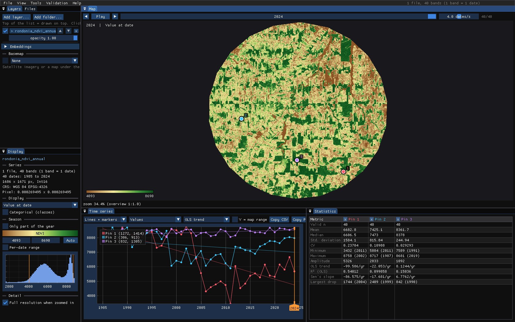
The Janus window with the 2024 NDVI of a circular area of Rondônia, forest in dark green and pasture in light colours, three pins on the map and their forty-year series on the chart. — **The series in 2024**, forest in dark green, and three pins: a forest cleared in the early 2000s, one cleared in 1999 that grew back, and a forest that stood throughout.

The stack is one GeoTIFF with a band per year, named yr1985 to yr2024: Janus reads the years from the band names. Outside the circle the file holds 0, so it is opened through a VRT that declares 0 as no data; otherwise the edges would be read as an NDVI of 0.

03Opening the tool

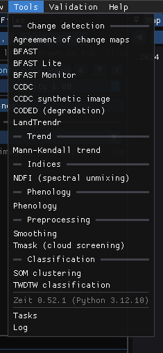
The Tools menu: change detection (agreement, BFAST, BFAST Lite, BFAST Monitor, CCDC, CCDC synthetic image, CODED, LandTrendr), trend, indices, phenology, preprocessing and classification tools, then Tasks and Log. — **Tools menu.** The Zeit tools by category.

Tools → Change detection → LandTrendr opens its window. The tools come from Zeit, whose methods are part of Janus: nothing to install. A tool that does not fit the series open is disabled, with the reason (LandTrendr on a monthly series: it needs one date per year).

04On the chart

With Fit the cursor, pins and ROI series ticked, LandTrendr runs on every exact series the chart shows, as you move the mouse or drop pins, and draws its segments and vertices over them. Its numbers go to the Statistics table.

LandTrendr's window with its parameters on the right; on the chart the NDVI of the cleared pixel with the fitted segments in magenta; the Statistics table with the vertices, segments and the mapped event. — **The cleared forest.** Stable near 0.82 until 2002, down to 0.38 by 2009, slowly up since: one loss segment.

The chart: the yearly NDVI of the pixel and the LandTrendr fit, a flat segment, a steep drop from 2002 to 2009 and a slow rise. — **The fit**: vertices as dots, segments as lines.

The Statistics table: 6 vertices, 5 segments, 1 loss segment, mapped event 4465.4 from 2002 to 2009, pre 8251.5 and post 3786.1. — **Its numbers**: the mapped event is the 2002–2009 loss of 4465 (0.45 NDVI).

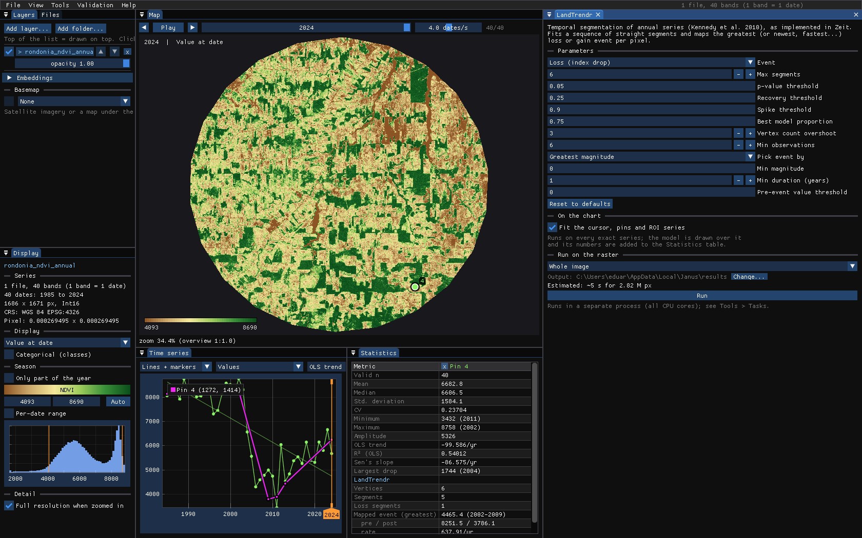
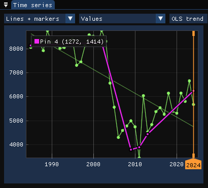
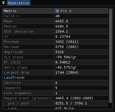
The table reads: 6 vertices and 5 segments, of which 1 is a loss; the event a map would show is the greatest loss, 4465.4 from 2002 to 2009, from 8251.5 to 3786.1. The other segments are the noise around the pasture and its slow gain, smaller than the loss.

Fit first, run later

The chart is where parameters are chosen: drop pins on the cases you know (a clearing, a regrowth, a forest that should stay untouched, a field) and change the parameters until each reads as it should. The run on the image uses exactly what the window shows.

05The parameters

Loss or gain

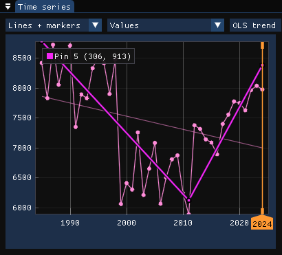
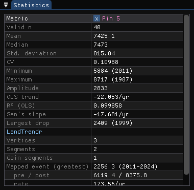
Event sets the direction of interest: Loss for a drop of the index, Gain for a rise. It orients the segmentation and which segments become events. On the pixel cleared in 1999 that grew back, looking for gains maps the regrowth:

The chart of the regrowth pixel: a long decline to 2011 and a rise to 2024, fitted with two segments. — **Gain** on the regrowth: down to 2011, up since.

The Statistics table: 3 vertices, 2 segments, 1 gain segment, mapped event 2256.3 from 2011 to 2024. — The mapped gain: **2256** (0.23 NDVI), 2011–2024.

How many segments

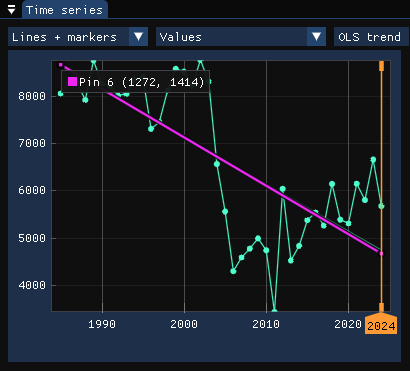
Max segments limits how detailed the trajectory can be. Too few and real events are lost: with two segments at most, the cleared pixel becomes one long decline from 1985 to 2024, with no year of clearing at all.

The chart of the cleared pixel fitted with at most two segments: a single straight decline over the whole series. — **Max segments 2**: the clearing disappears into a straight line.

All of them

Parameter	Default	What it does
Event	loss	Direction of interest: a drop or a rise of the index.
Max segments	6	The most segments the trajectory may have.
p-value threshold	0.05	Models with a worse p-value are rejected (simpler ones are tried).
Recovery threshold	0.25	The fastest recovery allowed, per year (1 / years): faster rises are taken as noise, not as regrowth.
Spike threshold	0.9	Dampens single-year spikes (a missed cloud); 1 keeps them.
Best model proportion	0.75	Prefers the model with the most vertices whose p-value is close enough to the best one.
Vertex count overshoot	3	Extra candidate vertices found before the weakest are pruned.
Min observations	6	Pixels with fewer valid years are not fitted.
Pick event by	greatest	Which event a pixel's maps show when it has several: the greatest, newest, fastest, longest, or the clearest (DSNR).
Min magnitude	0	Events smaller than this are ignored, in the units of the series.
Min duration	1	Events shorter than this (years) are ignored.
Pre-event value threshold	0	Loss: only events that start above this value (a forest); gain: below it. 0 is off.

The first eight shape the segmentation; the last four only choose which event is mapped. Thresholds are in the units of the series: here NDVI × 10000, so a minimum magnitude of 2500 is a drop of 0.25 NDVI.

06Running it on the image

Under Run on the raster, choose the scope: the Whole image, the Visible area of the map, or the ROI. Janus estimates the run time from a sample of the series (here about 6 s for 2.8 million pixels). Run starts the run in the background on every core; its progress is in Tools → Tasks, and the map stays usable meanwhile.

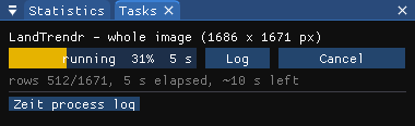
The Tasks panel: LandTrendr on the whole image, 1686 by 1671 pixels, running at 31 percent, 512 of 1671 rows, about 10 seconds left, with the Log and Cancel buttons. — **Tasks**, while the run goes: rows done, time left, Log and Cancel. Once done, Folder opens its outputs.

For the map, only real clearings should count: the run used a minimum magnitude of 2500 (0.25 NDVI) and a pre-event value of 7500 (the loss has to start in forest). Without them every pixel gets some loss, if only a dry year in the pasture.

The outputs are GeoTIFFs (in %LOCALAPPDATA%\Janus\results by default, next to the run's job.json and job.log), opened over the map as layers of their own in the Layers panel (hide the series and the panel under the map shows every map's value at the cursor and the pins, the histogram and the area of each year). Pixels without an event are transparent.

07The maps

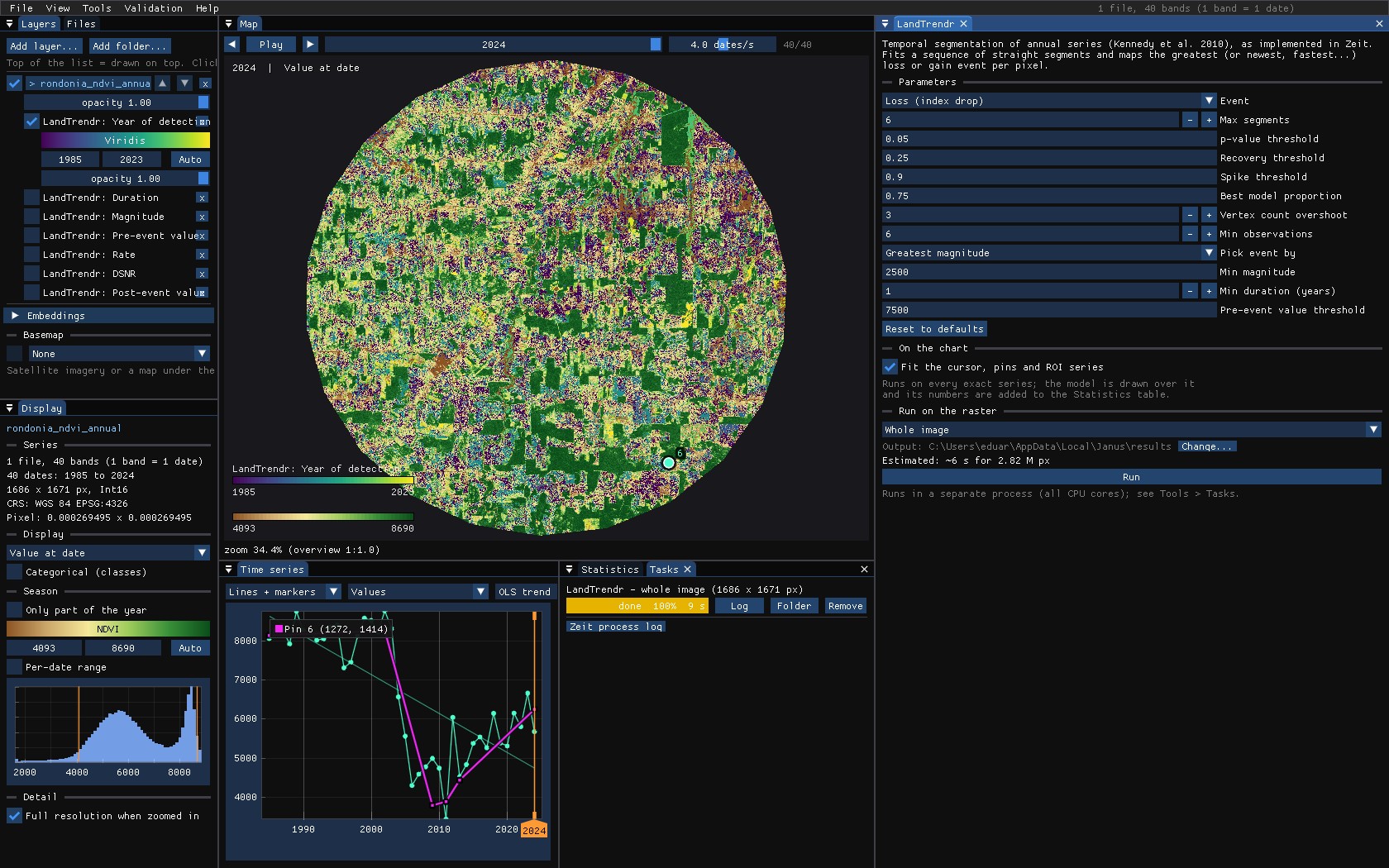
The year of detection over the circle: purple for losses of the 1980s and 1990s, green and yellow for recent ones, with the forest left without colour; the Layers panel lists the seven outputs. — **Year of detection**, 1985 (purple) to 2023 (yellow). The forest that stood shows through in dark green.

Each output is a layer with its own colour scale and range, which you can hide, reorder, export as GeoTIFF or compare with a swipe:

Map	Meaning
Year of detection	The year the mapped event starts.
Magnitude	How far the index moved over it.
Duration	Its length in years: a clearing is 1–2, a slow decline many.
Pre-event / post-event value	The index at the start and at the end of the event.
Rate	Magnitude per year.
DSNR	Magnitude over the fit's error: low values are events barely above the noise.

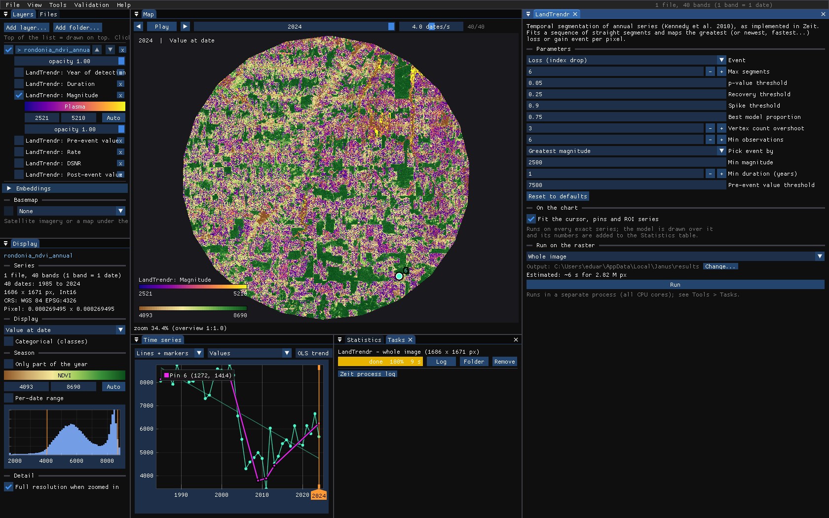
The magnitude of the mapped loss, from 2521 to 5210, over the same area. — **Magnitude** of the same events: the deepest clearings in yellow.

Hover the map with a result on top: the chart still shows the pixel's series and its fit, so every colour can be checked against the trajectory behind it.

08Recovery

The maps above say when a forest was lost. Tools → Change detection → Recovery (LandTrendr) asks what came after: it segments each series as LandTrendr does, takes the greatest loss as the disturbance, and measures the fitted trajectory after its lowest point, the trough. Measured on the fit, not on the yearly values, a dry year or a missed cloud does not end a recovery.

Pre-disturbance value: The mean of the years just before the disturbance (2 by default).
Y2R: Years to recovery: from the trough until the fit first gets back to 80% of the pre-disturbance value (White et al. 2017). 0 when it never fell below that; no value when it has not got back by the last year.
ARI: Absolute recovery: how much the fit rose from the trough after 5 years (the horizon), in the units of the series.
RRI: Relative recovery: ARI over the magnitude of the loss. 1 is all of it back.
R80P: The value after 5 years over 80% of the pre-disturbance value. 1 or more is recovered.
YrYr: Year-on-year recovery: the rise from the trough to year 5, per year.

The value after the horizon is the best of the fitted values of years 4 and 5 after the trough (Frazier et al. 2018). On the chart, the tool draws the LandTrendr fit, the recovery level as a dashed line from the trough, and a vertical line at the year the pixel recovered.

Two pixels

The tool was set as the LandTrendr run of section 06: a minimum magnitude of 2500 and a pre-event value of 7500, so that only clearings of forest count as disturbances. The forest cleared in 1998–1999 that grew back:

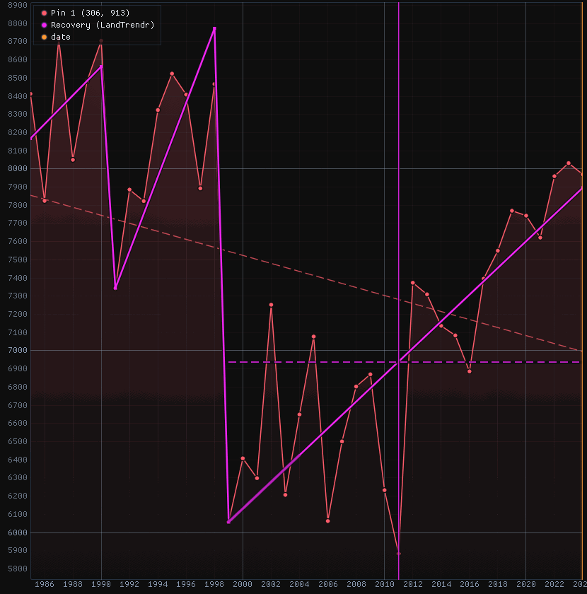
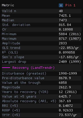
The chart of the regrowth pixel: NDVI near 8500 until 1998, down to about 6000 in 1999, then a fitted rise that crosses the dashed recovery level at 6937 in 2011, where a vertical line marks it, and goes on to about 7900 by 2024. — **Recovered in 2011**: the fit crosses the dashed 80% level 12 years after the trough.

The Statistics table of the recovery: disturbance 1998-1999, pre-disturbance value 8670.9, value at the trough 6058, magnitude 2612.9, years to recovery 12 (2011), value at +5 years 6425.7, ARI 367.69, RRI 0.14072, R80P 0.92633, YrYr 73.537 per year. — Its numbers: Y2R 12, R80P 0.93, RRI 0.14.

Before the clearing the fit stood at 8670.9 (its mean over 1997 and 1998); the trough is 6058 in 1999, a loss of 2612.9. Five years later the fit had risen by 367.7 (ARI): 14% of the loss (RRI), 93% of the way to the recovery level of 6936.7 (R80P), 73.5 a year (YrYr). It got there in 2011: Y2R = 12.

The forest cleared from 2002 to 2009 and kept as pasture:

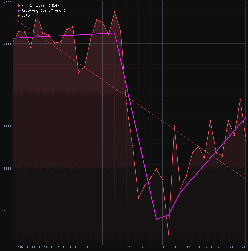
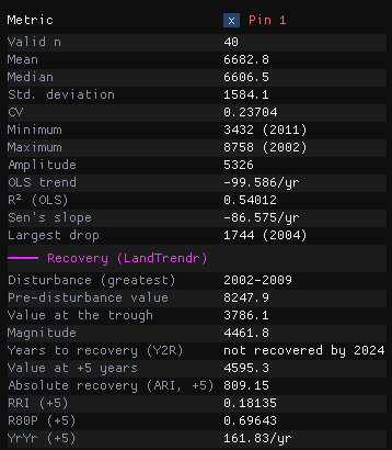
The chart of the pasture pixel: NDVI near 8200 until 2002, a fitted drop to about 3800 in 2009, then a slow rise to about 6200 by 2024, still under the dashed recovery level near 6600. — **Not recovered**: the fit stays under the dashed level to the end.

The Statistics table: disturbance 2002-2009, pre-disturbance value 8247.9, value at the trough 3786.1, magnitude 4461.8, years to recovery: not recovered by 2024, value at +5 years 4595.3, ARI 809.15, RRI 0.18135, R80P 0.69643, YrYr 161.83 per year. — Y2R: **not recovered by 2024**.

Here the loss is 4461.8, and the pasture's slow rise gives a larger ARI (809.2) and YrYr (161.8 a year) than the regrowth's, but only 18% of the loss (RRI) and 70% of the recovery level after five years (R80P). The level, 6598.3, is never reached: the pixel has no Y2R. Read the metrics together: a fast early rise is not a forest coming back.

The parameters

The tool has LandTrendr's parameters (section 05), which find the disturbance, and four of its own:

Parameter	Default	What it does
Horizon (years)	5	Years after the trough at which ARI, RRI, R80P and YrYr are measured.
Recovered at (fraction)	0.8	The fraction a pixel must get back to: 0.8 for White et al.'s Y2R and R80P.
Recovery level	pre-disturbance value	Fraction of the pre-disturbance value, for an index that is positive and drops (NDVI, NBR); or Fraction of the loss regained, for any index and either direction (gains need this one).
Pre-disturbance years	2	Years averaged for the pre-disturbance value, up to the start of the disturbance.

The maps

Run on the whole image (about 10 seconds for its 2.8 million pixels), the tool writes eight maps: years to recovery, R80P, RRI, ARI, YrYr, and the disturbance's magnitude, pre-disturbance value and year. Of the image's 2.8 million pixels, 22.7% have a disturbance and 7.6% a years to recovery: the others had not got back to the level by 2024.

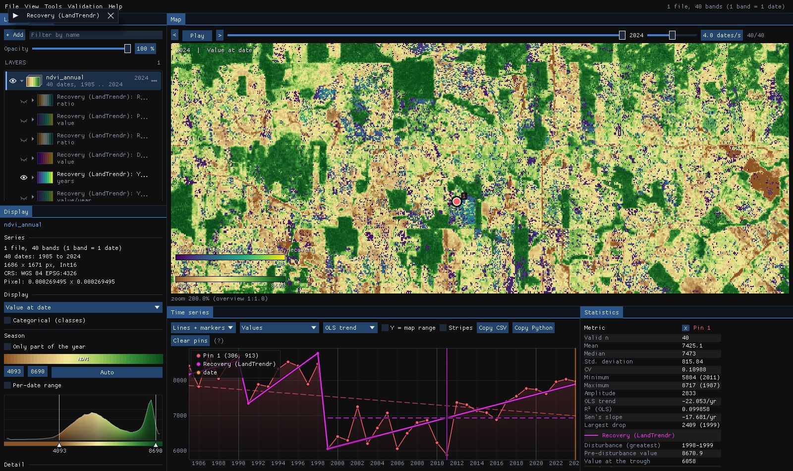
The years to recovery over the 2024 NDVI, zoomed in around the regrowth pixel: a patch of about 12 years in teal at the pin, scattered pixels of 1 to 5 years in purple over the pastures, and the forest and most pastures without a value. — **Years to recovery**, 1 (purple) to 38 (yellow), over the 2024 NDVI. The patch at the pin took about 12 years.

The scattered pixels of 1 to 5 years in the pastures are cases to check on the chart before believing: a loss barely past the thresholds whose fit gets back to 80% within the year-to-year noise. A higher Min magnitude, or the Pick event by and Min duration filters, leave them out.

Against the original

Zeit's recovery metrics agree with the R package RecoverMetricsR to float32's precision (a relative difference of 6e-8). On 1000 × 1000 pixels of 21 years, RecoverMetricsR takes 52.4 s and Zeit 98 ms on one thread, 535 times faster.

09What next

Validate it. The year of detection is a map of events: the Validation guide stratifies it, draws a sample and estimates its accuracy and the area of loss by year, with confidence intervals.
Compare it. Tools → Change detection → Agreement of change maps takes several maps of dates (LandTrendr, CCDC, BFAST, CODED) and maps where and when they agree.
Export it. Right click a result in the Layers panel to save it as GeoTIFF, or save the map as a PNG figure.
Script it. The same algorithm is zeit.landtrendr and zeit.extract_events in Python.

10References

Kennedy, R. E., Yang, Z., Cohen, W. B. (2010). Detecting trends in forest disturbance and recovery using yearly Landsat time series: 1. LandTrendr — Temporal segmentation algorithms. Remote Sensing of Environment, 114, 2897–2910.
Kennedy, R. E. et al. (2018). Implementation of the LandTrendr algorithm on Google Earth Engine. Remote Sensing, 10(5), 691.
Kennedy, R. E., Yang, Z., Cohen, W. B., Pfaff, E., Braaten, J., Nelson, P. (2012). Spatial and temporal patterns of forest disturbance and regrowth within the area of the Northwest Forest Plan. Remote Sensing of Environment, 122, 117–133.
White, J. C., Wulder, M. A., Hermosilla, T., Coops, N. C., Hobart, G. W. (2017). A nationwide annual characterization of 25 years of forest disturbance and recovery for Canada using Landsat time series. Remote Sensing of Environment, 194, 303–321.
Frazier, R. J., Coops, N. C., Wulder, M. A., Hermosilla, T., White, J. C. (2018). Analyzing spatial and temporal variability in short-term rates of post-fire vegetation return from Landsat time series. Remote Sensing of Environment, 205, 32–45.
Zeit: the change detection library behind the tools of Janus.

LandTrendr, step by step.