

01The idea
Counting the pixels of a class gives the mapped area. It is biased by the map's errors: every pixel of forest the map calls deforestation adds to it (commission), every clearing it misses takes from it (omission). To know the real area you need a reference: what is really on the ground at a set of places, from images better than the ones the map was made from, or from a closer look at them. A sample of places, chosen at random with known probabilities, lets you estimate from those few points the map's accuracy and the area of each class over the whole map, with a confidence interval.
Janus does each step of that in the same window where you look at the series:
- StrataSplit the map into strata: its classes, its dates of change, a buffer around change.
- Sample sizeHow many points, and how many in each stratum, for the precision you want.
- DrawA stratified random sample, saved as a project (a GeoPackage).
- InterpretEach point, blind to the map: its series, its images at every date, a label.
- EstimateOverall, user's and producer's accuracy, adjusted areas, all with intervals.
- ReportTables, figures and a methods paragraph, ready for the paper.
A few words used below
- Map
- The product being assessed: a land-cover map, a map of the year of change, a Zeit result.
- Reference
- The class (and the date of change) you give a sample point from the images. It is taken as the truth.
- Stratum
- A part of the map sampled on its own: each stratum gets its own number of points, drawn at random among its pixels.
- Weight
- A stratum's share of the map's area. The estimators weigh each point by it, so a stratum sampled more densely than its area does not bias the estimates.
- User's accuracy
- Of the pixels the map calls a class, the share that really is that class (1 − commission error).
- Producer's accuracy
- Of the area that really is a class, the share the map calls that class (1 − omission error).
- Adjusted area
- The area of a class estimated from the reference labels and the strata's weights, not from the map's pixel count; given ± its confidence interval.
02The example
The screenshots follow one validation from start to end. The map is the forest loss of 2018–2023 in Global Forest Change v1.11 (Hansen et al. 2013): for each pixel, the year it lost its forest, or nothing. The place is 16 × 13 km south-west of Novo Progresso, Pará, on the BR-163 deforestation front. The reference comes from Sentinel-2: one cloud-free composite per dry season, 2017 to 2024, with six bands (blue to SWIR2), opened as a series in Janus.
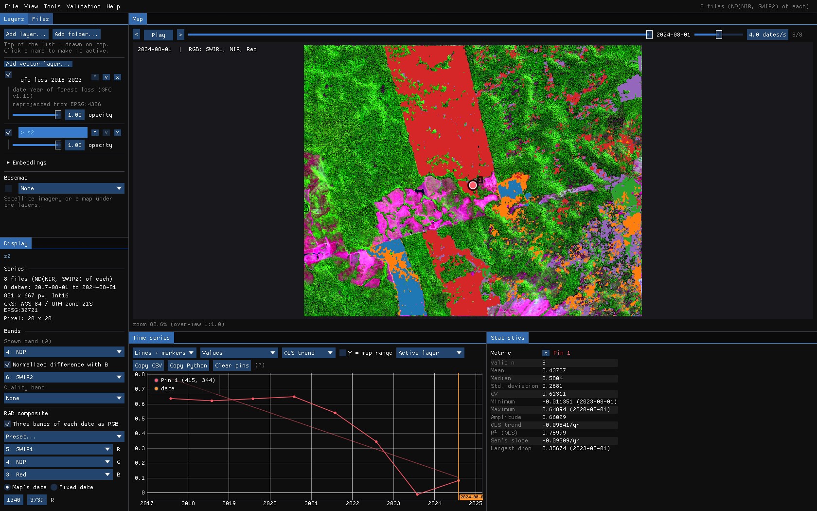
Open both as you would for any other work: the images with File → Open folder... (or jn on the command line), the map with File → Add layer: file(s).... Show the images in a composite that makes the change easy to see (the RGB composite of the Display panel), and the chart in an index that separates forest from what replaces it (here the NBR, the normalized difference of NIR and SWIR2). The map does not even need to be open: the design can read it from a file.
Reproduce it
python tools/make_tutorial_data.py data downloads the same area (about 60 MB, read in place from the public buckets of Earth Search, Global Forest Change and MapBiomas). janus --shots validation data out then runs this whole guide and saves these screenshots.
About the numbers
To keep the guide reproducible, the points in these screenshots were labelled by a simple rule on each point's NBR series (a drop from forest, and whether it grew back), not by a person looking at the images. The numbers show how to read the tool; they are not an assessment of Global Forest Change.
03The Validation menu
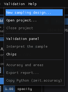
- New sampling design... opens the Validation panel on its Design tab: the strata, the sample size, the draw.
- Open project... reopens a project saved before (the GeoPackage), with its labels; work resumes where it stopped. Close project saves what is pending.
- Validation panel, Interpret the sample and Chips show the three panels you work in.
- Accuracy and areas goes to the results; Export report... writes them to a folder; Python (zeit.accuracy)... shows the
zeit.accuracycode that computes the same numbers from the project's files, in an editor to copy or save it.
The Validation panel has five tabs, in the order of the work: Design, Accuracy, Maps, Interpreters and Report.
04Maps to stratify
Strata are what make a sample efficient. Change is usually rare: in a simple random sample of 300 points over a map with 2% of loss, about six would fall on loss, too few to say anything about it. Sampling each stratum separately lets you put 50 or 100 points on the rare classes and still estimate everything without bias, because each point counts by its stratum's weight.
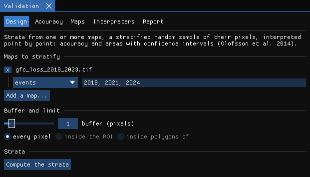
Add a map
Add a map... lists the maps already open (Zeit results, layers at their date) and A raster file.... Then say how its values are read:
- classes: each value is a class (a land-cover map, a TWDTW or SOM result). Its classes become the strata. Tick the ones that are change; that matters for the buffer and for several maps.
- intervals: ranges of a continuous value, with their edges, e.g.
-1, -0.1, 1for a magnitude, and which ranges are change. - events: the value is the date of a change (LandTrendr's year of detection, a loss year). Above zero is change; zero and no data are not. With periods (
2018, 2021, 2024), each period becomes a stratum of its own: here 2018–2020 and 2021–2023.
With several maps, the strata are their agreement: one stratum for each number of maps that call a pixel change (change in 2 of 3 maps...). A good design when you will compare the maps later.
Buffer
The pixels without change within N pixels of a change become a stratum of their own. The changes a map misses are mostly next to the ones it found (the edge of a clearing mapped too small, a clearing of the year after). Without a buffer those few omission errors fall in the huge stratum of no change, where each point weighs a lot, and they inflate the interval of the area of change. A handful of points in the buffer makes the area much more precise (Olofsson et al. 2020).
Limit
every pixel of the map, inside the ROI drawn on the map, or inside polygons of a vector layer you opened (a municipality, a biome, a study area).
05The strata
Compute the strata reads the map once at full resolution, in the background. The result is a raster of strata, opened as a layer, and a table with each stratum's pixels, area (in hectares, on the sphere for a geographic CRS like this one) and weight.
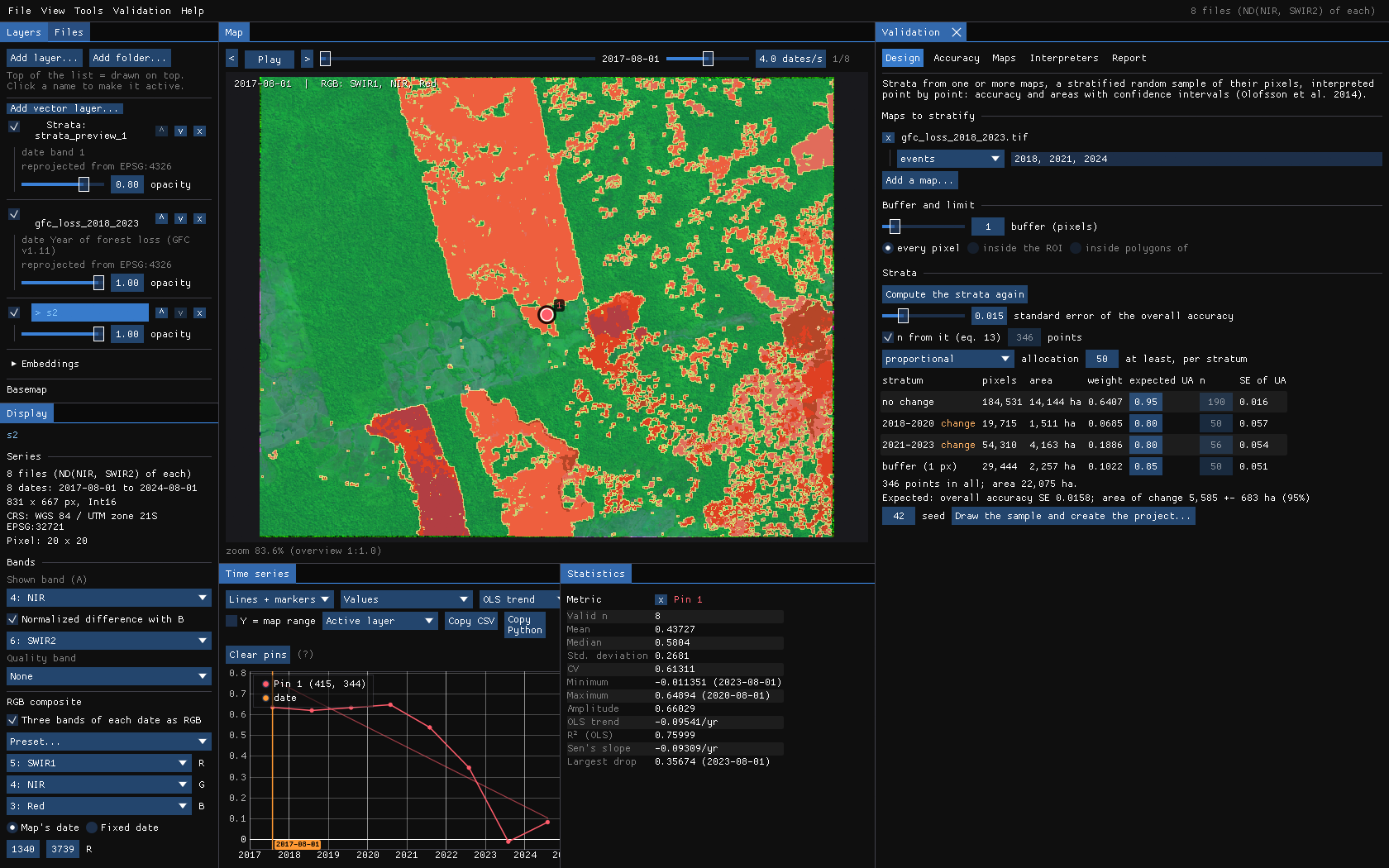
If you change the maps, the buffer or the limit afterwards, the panel says so (the maps or the limit changed) and the sample cannot be drawn until the strata are computed again.
06Sample size and allocation
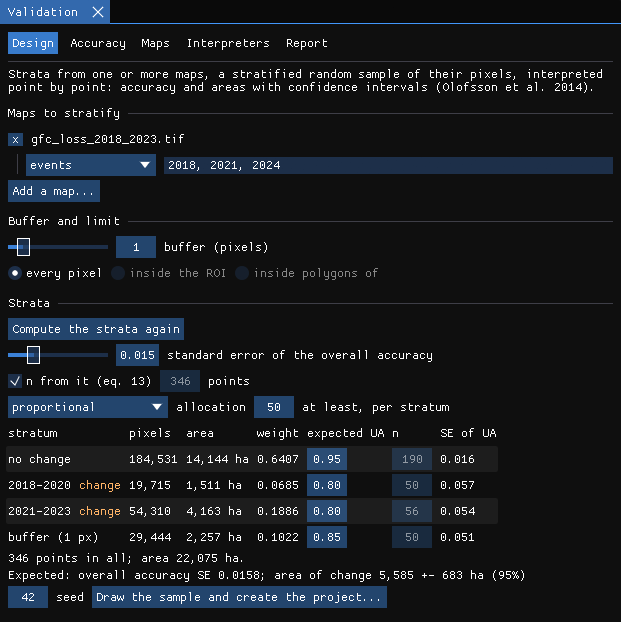
- Standard error of the overall accuracy: the precision you want. With n from it (eq. 13) ticked, the number of points comes from equation 13 of Olofsson et al. (2014), from the strata's weights and the user's accuracy you expect of each. Untick it to give the number yourself.
- Expected UA (in the table): the user's accuracy you expect of each stratum. Hard classes (change) 0.6–0.8, easy ones 0.9–0.95. It sets n and the Neyman allocation; guess from a quick look, or from a pilot sample.
- Allocation: proportional to the strata's areas, equal in each, Neyman (to area × the expected standard deviation), or by hand in the n column. With at least, per stratum, the rare strata get a floor: Olofsson et al. advise 50 to 100 points for the accuracy of a rare class.
Under the table, Janus shows the errors this design should give if each stratum's accuracy is as expected: the standard error of each user's accuracy, of the overall accuracy, and the interval of the area of change. Change the numbers until those are good enough for your purpose, before drawing anything.
07Drawing the sample
Draw the sample and create the project... asks where to save the project, a GeoPackage, and draws the points at random among each stratum's pixels, at the pixels' centres. The strata raster is saved beside it. The seed makes the draw repeatable: the same strata, sizes and seed always give the same points.
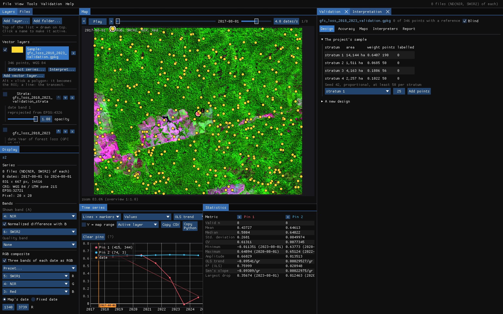
The project is an ordinary GeoPackage; open it in QGIS, keep it with the paper's data. Its tables are samples (the points, with the reference label of each once there is one), labels (every label of every interpreter, with its date, confidence and notes), strata and project (the design, the maps assessed and how their classes read the labels).
The interpretation starts at once, blind: the maps being assessed and the strata are not drawn, and the points are coloured only by their state. Knowing what the map says sways the reference toward it; the blind mode keeps that from happening. Blind is a checkbox in the panel; it is better left on until the last label.
Later, Add points (top of the Design tab) draws more points in one stratum, among its pixels not yet sampled. The sample stays a stratified random sample: useful when a rare class's accuracy is still too uncertain.
08Interpreting the points
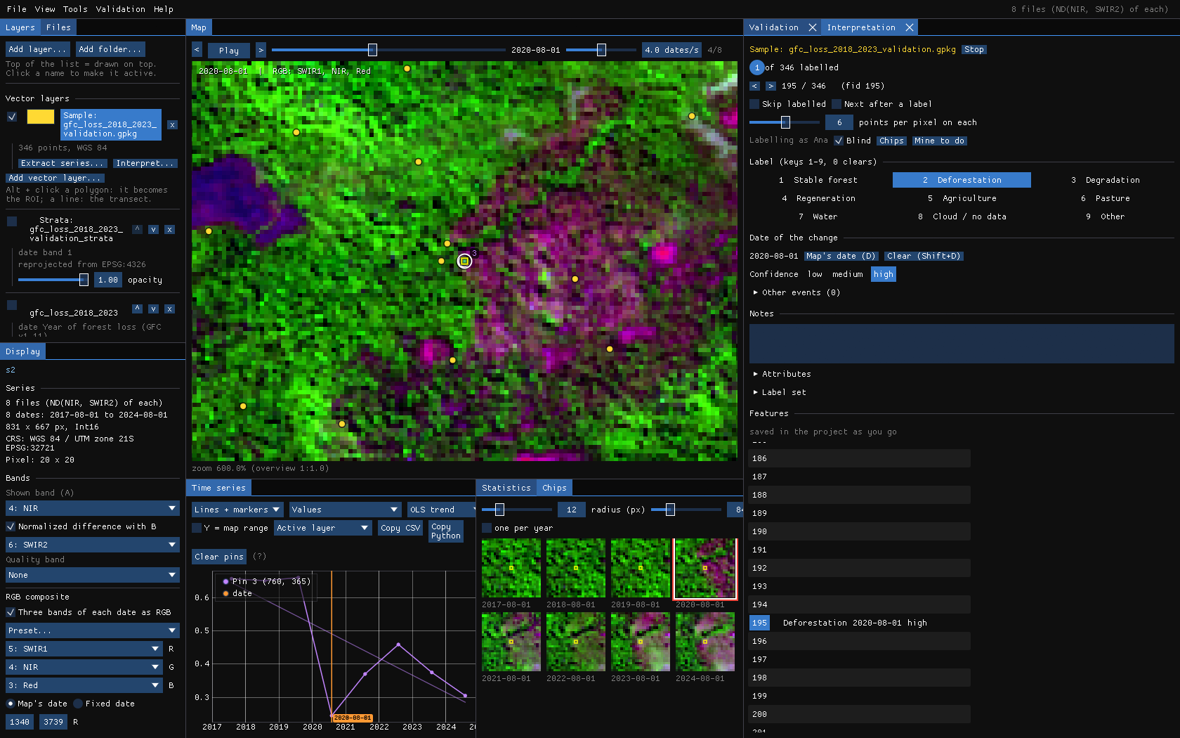
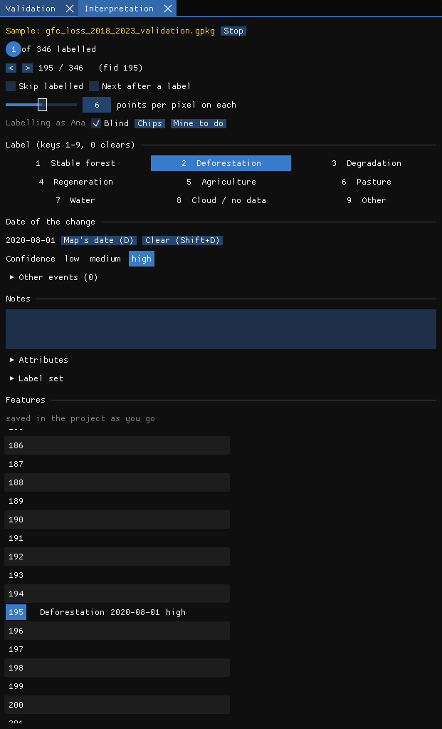
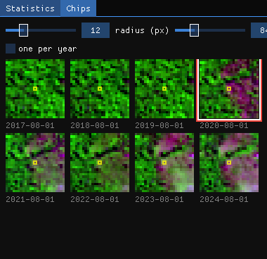
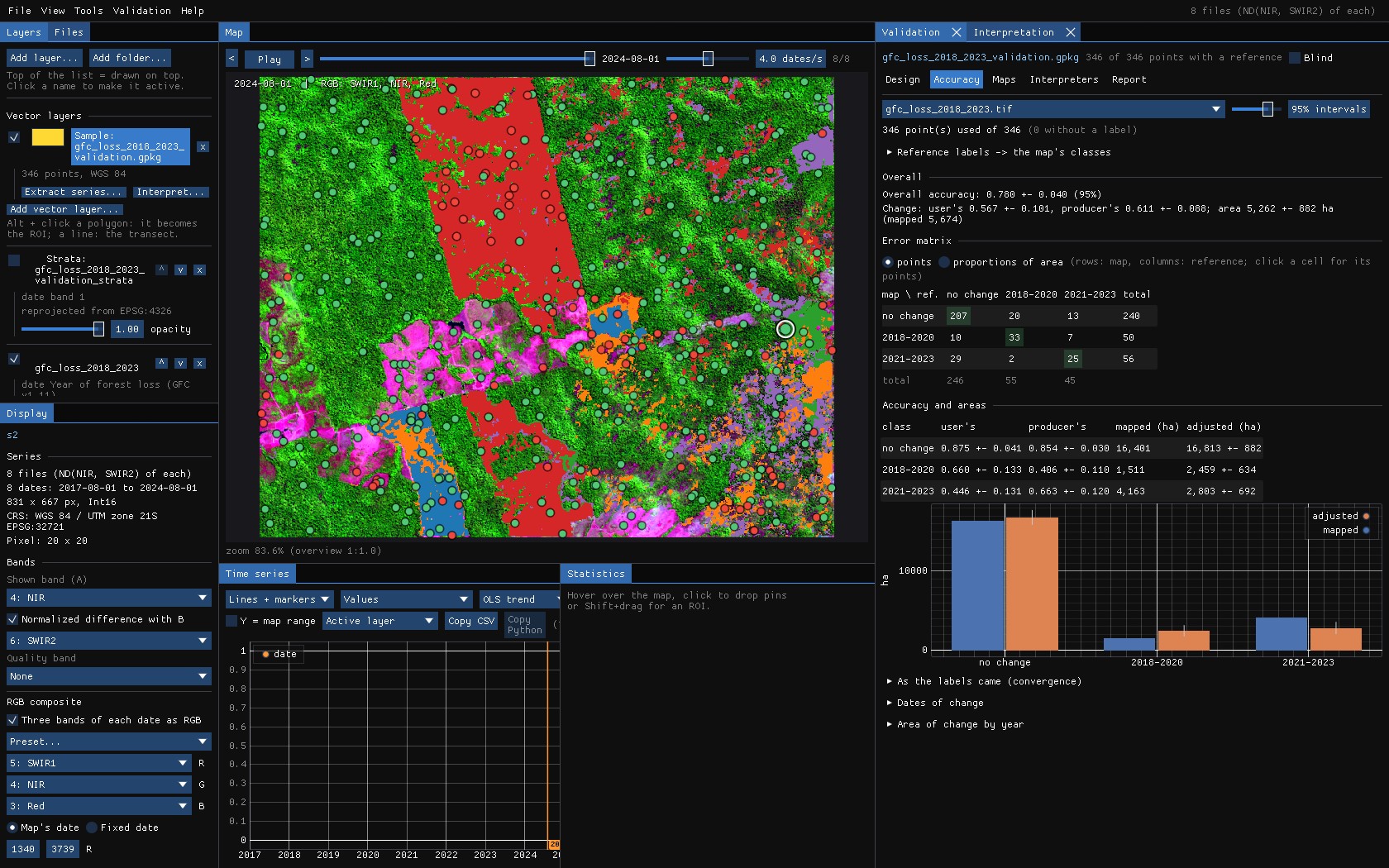
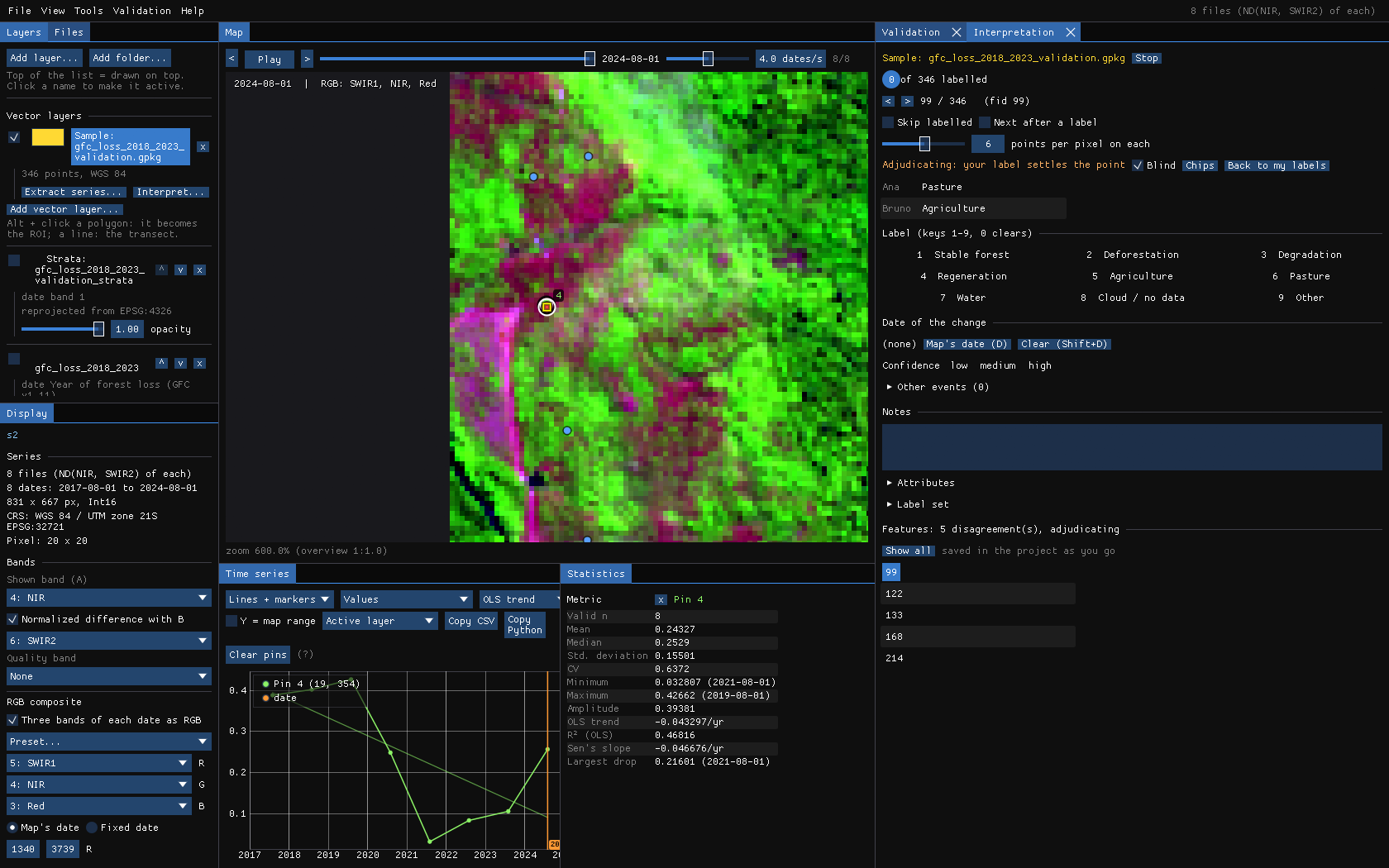
The Interpretation panel takes the points one by one, as TimeSync does. The map goes to each point and outlines its pixel, the chart shows its series (a pin), and the Chips panel shows a small window around it at every date.
The keys
| Key | What it does |
|---|---|
| N / Shift+N | Next / previous point (also Page Down / Page Up). Mine to do keeps only the points you have not labelled. |
| 1–9 | A label of the label set: Stable forest, Deforestation, Degradation, Regeneration, Agriculture, Pasture, Water, Cloud / no data, Other (edit it under Label set). 0 clears it. |
| ← / → | The previous / next date on the map; a click on the chart or on a chip goes to its date. |
| D | The date of the change is the date on the map (double click a chip does the same). Shift+D clears it. |
| Shift+1 / 2 / 3 | Confidence: low, medium, high. |
| E | Another event at the map's date: a point degraded in 2019, then cleared in 2022, keeps both. |
Label what is on the ground, not what the map says: the class, and for a change the date it shows up. Labels are written to the GeoPackage a second after each change, so closing Janus loses nothing. If an image cannot tell (clouds, a pixel on an edge), say so with Cloud / no data or Other and a note: those points are left out of the estimates, and the report counts them.
Chips
The chips use the active layer's colours, or its RGB composite. One per year keeps the date nearest the map's day of the year when the series has many dates. The next points' chips are read ahead, so moving on with N is immediate.
09Accuracy and areas
The Accuracy tab is recomputed with every label: you can watch the estimates settle as you go. Choose the map at the top (a project can assess several) and the confidence level of the intervals (95% by default).
Reading it
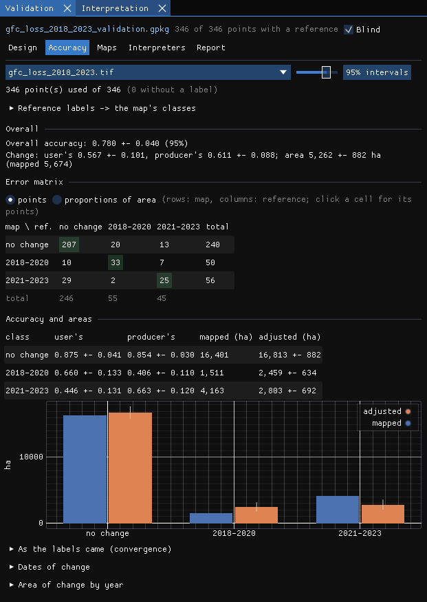
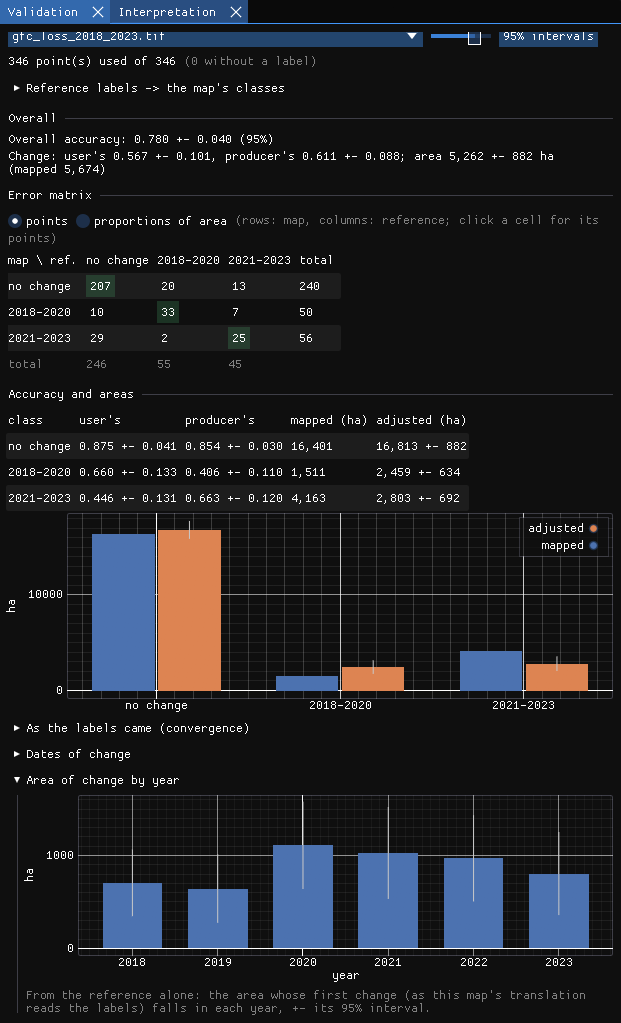
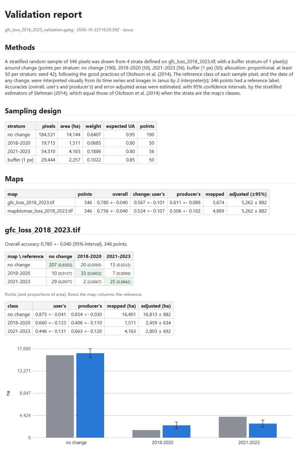
- Overall accuracy 0.780 ± 0.040: the share of the map's area that is right, ± the half-width of its interval.
- Change: the user's accuracy of change 0.567 ± 0.101 (of what the map calls loss, how much is loss), its producer's accuracy 0.611 ± 0.088 (of the real loss, how much the map found), and the adjusted area of change, 5,262 ± 882 ha, against the 5,674 ha the map counts.
- The error matrix: rows are the map, columns the reference. In points it counts the sample; in proportions of area each cell is the estimated share of the map's area, the matrix the estimators work on. Click a cell and the Interpretation panel lists its points, so you can go through the errors one by one and check your labels.
- Accuracy and areas: for each class, user's and producer's accuracy, the mapped area and the adjusted area ± its interval, also as a chart. When the interval of the adjusted area does not contain the mapped area, the map's pixel count is biased beyond chance.
In the example, the total area of loss the map counts (5,674 ha) is inside the interval of the adjusted area, but the two periods are not. The map has 1,511 ha of loss in 2018–2020 where the reference estimates 2,459 ± 634 ha: it misses early loss (producer's accuracy 0.41). It has 4,163 ha in 2021–2023 against 2,803 ± 692 ha: a good part of what it dates to those years is not loss in the images, or is older loss (user's accuracy 0.45). The total looks right only because the two errors cancel out, and only the strata by period show it.
From labels to the map's classes
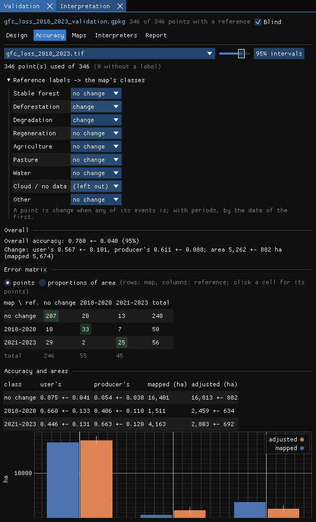
The label set describes the ground; the map has its own classes. Reference labels → the map's classes says how each label reads for this map. Janus guesses it from the names; for a map of events, loss and disturbance labels are change. Labels like Cloud / no data are left out.
The estimator of the areas
Areas by the ... estimator chooses how the adjusted areas are computed from the points:
- Direct (the default): the sample alone, each stratum's share of points with the class weighed by the stratum's area (Olofsson et al. 2014; Stehman 2014).
- Difference: the map's own area of the class, corrected by its net error estimated at the points (where the reference has the class minus where the map has it).
- Ratio: the map's area times the estimated ratio of the reference's share to the map's. It needs points the map calls the class.
The last two are model-assisted (Stehman 2013; McRoberts et al. 2018): they use the map's pixel count, known without error, and estimate only its error. When the strata are the map's classes the three give the same numbers. When they are not (a second map assessed with the same sample, the transitions below, a buffer stratum mixing classes), a good map gives much narrower intervals with them. The accuracies do not depend on the estimator; the choice is kept in the project, and the report and Copy Python use it.
10More from the labels
As the labels came
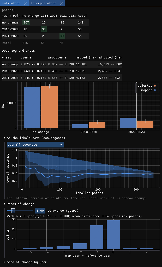
The estimate, and its interval, after each step of the labelling. It answers have I labelled enough?: when the interval of what you need (the overall accuracy, or the area of a class) is narrow enough, you can stop, or add points where it is still wide.
Dates of change
For a map of events, the points both the map and the reference call change are compared by date: the share within ± k years (the tolerance) and the histogram of the differences. Here the reference year is the first dry-season image that shows the clearing, so a loss mapped in a given year often shows in the next image: the histogram leans to −1.
Area of change by year
From the reference alone: the area whose first change falls in each year, ± its interval. The map's dates are not used, only its strata, so this is the series of loss to report, with the uncertainty that comes with it.
Transitions between two dates
With two maps of classes in the project (two dates of a categorical series, such as MapBiomas in 2000 and in 2020), Transitions between two dates in the Accuracy tab estimates the area of each transition, Forest -> Pasture, Forest -> Forest..., with its interval. The mapped areas are counted pixel by pixel inside the strata, in the background. The reference of each point at each date comes from its label and its dated events: the label holds until the first event with one of the maps' classes, which holds from its date on. A forest labelled Forest with an event Pasture in 2012 is Forest -> Pasture between 2005 and 2020, and Forest -> Forest between 2005 and 2010. The dates are guessed from the maps' names; type them if they are not right.
The table gives each transition's mapped and adjusted area ± its interval and its user's and producer's accuracy; only changes hides the classes that stayed. The sample need not have been stratified by the transitions: the points are weighed by the project's strata. Rare transitions are where the difference estimator helps most. Python... gives the zeit.transitions code that computes the same numbers.
Right and wrong on the map
Once the interpretation is done, untick Blind: the map and the strata come back, and in the Interpretation panel the points can be coloured by stratum or right / wrong for the selected map. The errors often cluster (along roads, at the edges of clearings), which tells you where the map struggles.
11One sample, many maps
The reference labels describe the ground, so the same sample can assess any other map of the same area: another product, a LandTrendr or CCDC result, last year's version of your own map. In the Maps tab, Assess another map... adds one; it is read at the points and its areas over the project's strata. The estimators weigh the points by the strata the sample was drawn from (Stehman 2014), so a map other than the one stratified is assessed without bias, only less precisely.
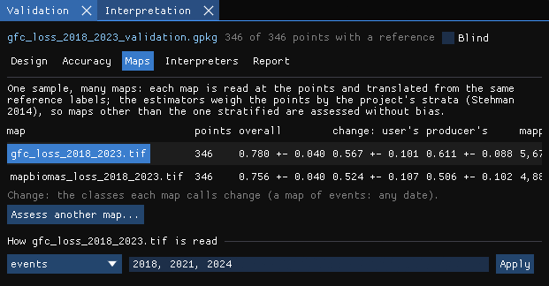
Here the second map is the loss of forest in MapBiomas Collection 9 over the same years. Note the last column: the adjusted area of change is the same for both maps, 5,262 ± 882 ha. It comes from the reference labels and the strata, not from the map, so a better map does not change the estimate of the area; it changes how far its own pixel count is from it (5,674 ha for one, 4,889 ha for the other).
Click a map's name to see its Accuracy tab; set how it is read (classes, intervals, events and their periods) under the table.
12Several interpreters
Two people reading the same images do not always agree, and how often they agree is worth reporting. Labels are kept by interpreter: your name is in File → Settings... (by default your login). Save a copy for an interpreter... writes a copy of the project (with its strata raster) for a colleague to label in their own Janus; Merge labels from a copy... brings their labels back, point by point, the newer kept.
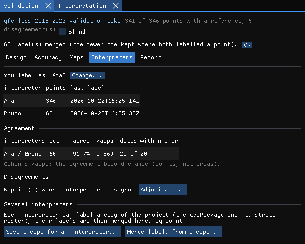
The tab shows each pair's agreement on the points both labelled, Cohen's kappa (the agreement beyond chance) and how often their dates are within a year. Adjudicate... goes through the disagreements: the others' labels are shown, and the label you give settles the point (it is kept as the adjudicated label, theirs stay as they were).
13The report
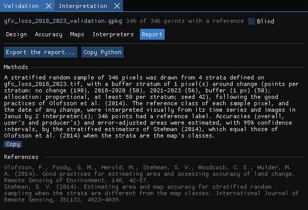
The Report tab writes a methods paragraph from the project (the strata, the points per stratum, the allocation, the seed, the number of interpreters and of labelled points, the estimators), with its references, ready to copy into a paper.
Export the report... writes to a folder a report.html (the design, the comparison of the maps, each map's error matrix, accuracies and areas with figures, the area of change by year, the transitions between two dates, the interpreters' agreement, the methods and the references) and a CSV of every table (transitions.csv for the transitions), for your own figures.
Python... shows the zeit.accuracy (and zeit.transitions) call that computes the same estimates, by the same estimator, from the project's GeoPackage and rasters: a check that does not depend on Janus, and a start for scripts of your own.
14Against official alerts
A sample tells how right a map is. A quicker question, before any sample, is how a map of change compares with the alerts the agencies publish: INPE's DETER in Brazil, UMD's GLAD (Landsat and Sentinel-2) and Wageningen's RADD (Sentinel-1) across the tropics. Validation & uncertainty → Official alerts... (the Alerts tab) puts the alerts on the grid of a map of change dates from a run (LandTrendr's year of detection, CCDC's or BFAST's break dates...) or from disk (decimal years, year and day, YYYYMMDD or days since 1970, the encoding detected) and says where and when the two agree. The alerts are another map, with errors of their own, so this is not an accuracy assessment: it shows where to look, and how early or late one map is against the other.
Here the map is LandTrendr's year of detection on the NBR of the eight composites (Tools → Change detection → LandTrendr, its defaults, the whole image), compared with the alerts of 2019 to 2023.
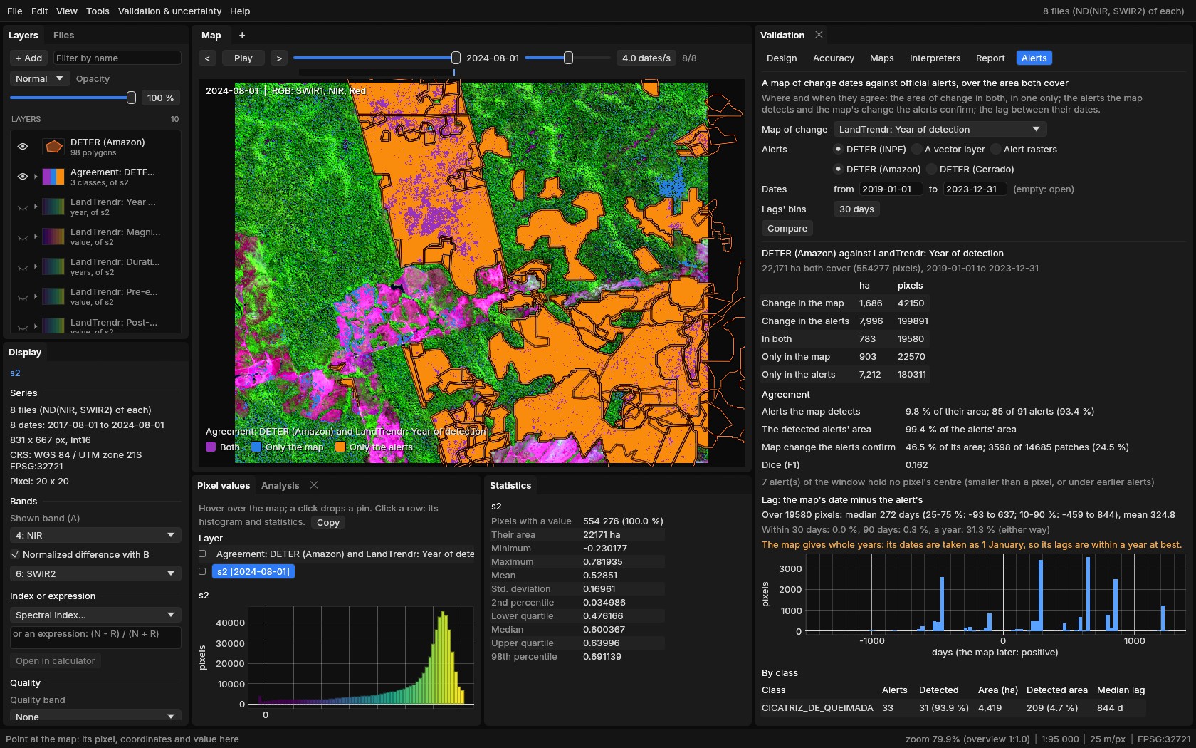
Choose the map, the source and the window of dates, then Compare. DETER comes from TerraBrasilis' public WFS, for the map's area only, and opens as a vector layer; GLAD's files are read straight from UMD's public bucket and RADD's from Global Forest Watch's map tiles, again for the map's area only (or from files you downloaded). Nothing needs a key.
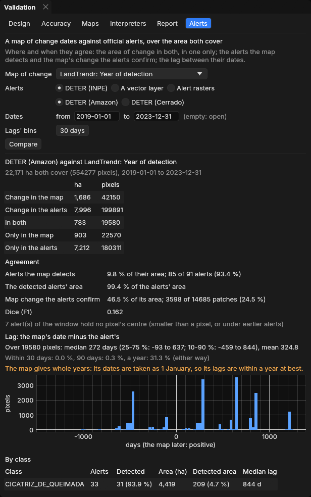
Reading it
- Areas: change in both, only in the map, only in the alerts, pixel by pixel over the area both cover.
- Alerts the map detects: an alert counts as detected when the map changed at one of its pixels at least. LandTrendr touches 85 of DETER's 91 alerts (93.4%), yet only 9.8% of their area: the polygons are much larger than the change LandTrendr finds inside them.
- Map change the alerts confirm: the share of the map's change inside an alert, by area (46.5% here) and by patch. Dice sums both sides up in one number (0.162).
- Lag: the map's date minus the alert's, in days, at each pixel in both. LandTrendr gives whole years, taken as 1 January, so its lags are within a year at best (the tab says so); a map of dates from a dense series (CCDC, BFAST) gives the real delay.
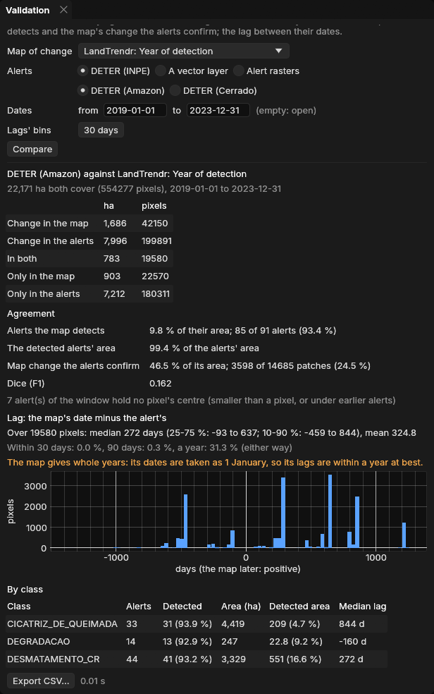
- By class: DETER's classes, or GLAD's and RADD's confidence.
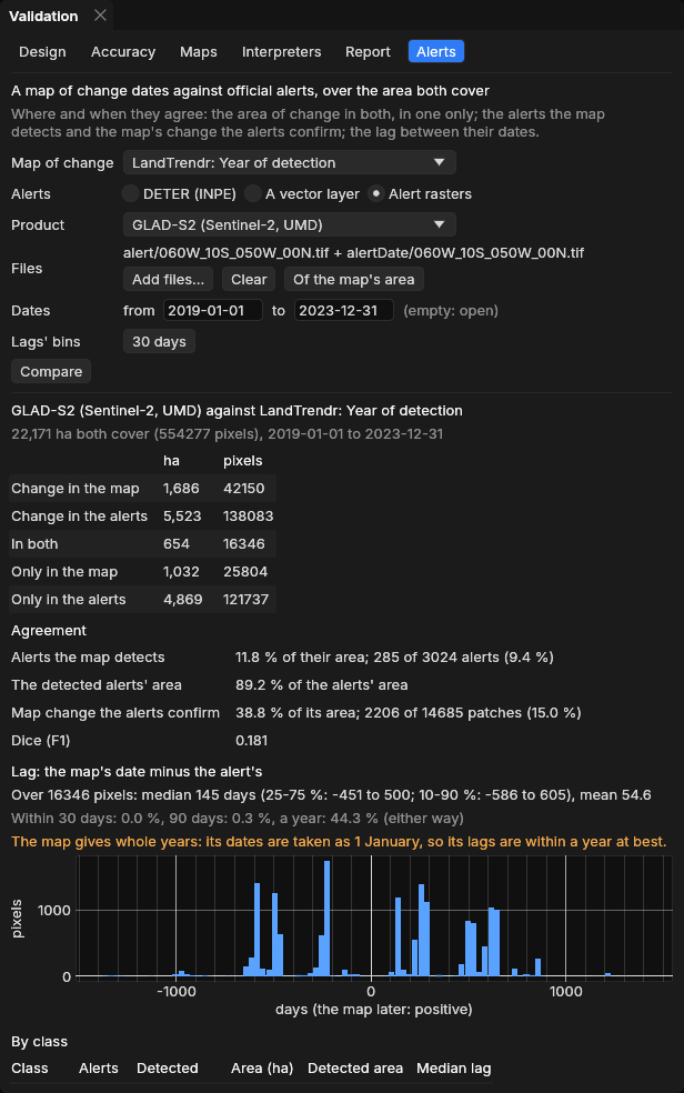
GLAD-S2 against the same map: 285 of its 3,024 alerts are detected (9.4%), but these hold 89.2% of the alerts' area: LandTrendr finds the large clearings and misses the many small alerts of a few pixels. 38.8% of the map's change is inside a GLAD-S2 alert.
Export CSV... writes the summary, the classes, every alert (its date, class, area and whether it was detected), the lags' histogram and the agreement map as a GeoTIFF. The rules, and a check of every number against geopandas, rasterio, numpy and scipy, are in the manual.
Reproduce it
With the guide's data, janus --shots alerts data out runs LandTrendr, fetches DETER and GLAD-S2 and saves these screenshots (it needs the network).
15Good practice
- Decide the design before looking at the results. Strata, sample size and seed are part of the method; drawing again until the numbers look good is not a random sample any more. To be more precise, add points in a stratum.
- Give rare classes enough points. 50 to 100 per stratum of change, whatever a proportional allocation would give them.
- Use a buffer for maps of change. It is where the omission errors hide.
- Stay blind. Untick it only when every point has a label.
- Use better data for the reference than for the map: a denser series, finer images, the basemap, field data. Interpreting the same images the map was made from mostly tells how well the algorithm read them.
- Report the intervals. An area of change is the adjusted area ± its interval, not the pixel count.
- Keep the project. The GeoPackage holds the points, every label and the design: anyone can recompute the estimates, in Janus or with
zeit.accuracy.
16References
- Olofsson, P., Foody, G. M., Herold, M., Stehman, S. V., Woodcock, C. E., Wulder, M. A. (2014). Good practices for estimating area and assessing accuracy of land change. Remote Sensing of Environment, 148, 42–57.
- Olofsson, P., Arévalo, P., Espejo, A. B., Green, C., Lindquist, E., McRoberts, R. E., Sanz, M. J. (2020). Mitigating the effects of omission errors on area and area change estimates. Remote Sensing of Environment, 236, 111492.
- Stehman, S. V. (2014). Estimating area and map accuracy for stratified random sampling when the strata are different from the map classes. International Journal of Remote Sensing, 35(13), 4923–4939.
- Stehman, S. V. (2013). Estimating area from an accuracy assessment error matrix. Remote Sensing of Environment, 132, 202–211.
- McRoberts, R. E., Stehman, S. V., Liknes, G. C., Næsset, E., Sannier, C., Walters, B. F. (2018). The effects of imperfect reference data on remote sensing-assisted estimators of land cover class proportions. ISPRS Journal of Photogrammetry and Remote Sensing, 142, 292–300.
- Hansen, M. C. et al. (2013). High-resolution global maps of 21st-century forest cover change. Science, 342, 850–853. Data: Global Forest Change 2000–2023 v1.11.
- Souza, C. M. et al. (2020). Reconstructing three decades of land use and land cover changes in Brazilian biomes with Landsat archive and Earth Engine. Remote Sensing, 12(17), 2735. Data: MapBiomas Collection 9.
- Sentinel-2 L2A: Copernicus Sentinel data, processed by ESA; cloud-optimized GeoTIFFs from Earth Search (Element 84).
- Kennedy, R. E., Yang, Z., Cohen, W. B. (2010). Detecting trends in forest disturbance and recovery using yearly Landsat time series: 1. LandTrendr — Temporal segmentation algorithms. Remote Sensing of Environment, 114(12), 2897–2910.
- Diniz, C. G. et al. (2015). DETER-B: The new Amazon near real-time deforestation detection system. IEEE Journal of Selected Topics in Applied Earth Observations and Remote Sensing, 8(7), 3619–3628. Data: INPE, TerraBrasilis.
- Hansen, M. C. et al. (2016). Humid tropical forest disturbance alerts using Landsat data. Environmental Research Letters, 11, 034008. Data: GLAD-L and GLAD-S2 alerts, GLAD laboratory, University of Maryland.
- Reiche, J. et al. (2021). Forest disturbance alerts for the Congo Basin using Sentinel-1. Environmental Research Letters, 16, 024005. Data: RADD alerts, Wageningen University, via Global Forest Watch.