Spectral unmixing

01The idea

Linear spectral mixture analysis (Adams et al. 1995) takes a pixel's reflectance in each band as the sum of the endmembers' reflectances, each weighted by the share of the pixel it covers. With a few endmembers and more bands than endmembers, the shares, or fractions, are what best rebuilds the pixel's spectrum. In the Amazon, the fractions of green vegetation, soil, dead vegetation and shade show logging and fire damage that a vegetation index misses (Souza et al. 2005).

Endmember: The spectrum of one pure material: dense vegetation, bare soil, water, shade. Here, a pin's bands on a place known to be that material.
Fraction: The share of an endmember in a pixel, from 0 to 1 with the default constraints.
FCLS: Fully constrained least squares (Heinz & Chang 2001): the fractions are not negative and add up to one. Each pixel is solved exactly.
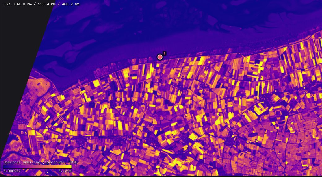
RMSE: The root mean square difference between the pixel's spectrum and the one the fractions rebuild, in reflectance. High where the endmembers do not describe the pixel.

02Two tools

Tool	Series	Endmembers	Outputs
Spectral unmixing (endmembers)	A multiband file per date (Landsat, Sentinel-2): every band of each date is read.	A pin's bands at the date shown.	A series of each fraction, their means over the dates, the mean RMSE and the number of observations unmixed.
Spectral unmixing (spectrum)	A hyperspectral scene, one band per wavelength (EnMAP, PRISMA, EMIT, AVIRIS).	A pin's spectrum.	A map of each fraction and the RMSE.

Both are under Tools → Spectral analysis, both run Zeit's unmix, and both are fitted live on the chart before they run on the image.

03The example

125 Landsat 8/9 dates of central Rondônia, Brazil, from February 2020 to August 2026: 1690 × 1675 pixels of 30 m, a GeoTIFF per date with the six reflectance bands (blue, green, red, NIR, SWIR1, SWIR2), clouds, shadows and snow already set to no data from the QA_PIXEL band. The scale and offset of Collection 2 (0.0000275 and −0.2) are in the files, so Janus reads reflectance.

The quality band

The tool reads every band of each date but the quality band. When the files carry one (QA_PIXEL, Fmask, SCL), choose it as the Quality band in the Display panel, with its rule: it masks the clouds and shadows of each date, which are then left out of the unmixing, and it is not unmixed itself. Here the files hold the six reflectances only, already masked.

04Endmembers from pins

Tools → Spectral analysis → Spectral unmixing (endmembers). Go to a clear date (here the last, 23 August 2026, in the dry season) and drop pins on pure covers: a dense forest, a field cleared to bare soil, open water. Add one from 2026-08-23... adds a pin's six bands at that date as an endmember; name each in its box.

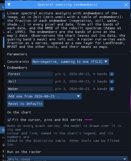
The Spectral unmixing (endmembers) window: constraints non-negative, summing to one (FCLS); three endmembers, Forest, Soil and Water, from pins 1, 2 and 3 at 2026-08-23 with 6 bands each; Add one from 2026-08-23; Fit the cursor, pins and ROI series ticked; Run on the raster: whole image. — **Three endmembers**, each the six bands of a pin on 23 August 2026.

Pick endmembers where the cover is pure over several pixels, and in the date you take them from: the soil pin here is a field cleared between 2020 and 2026, bare in August 2026 but forest in 2020. Two to six endmembers is usual; without the sum-to-one constraint, at most one fewer than the bands. Too many similar endmembers make the fractions unstable: the solver can trade one for the other at little cost.

05On the chart

With Fit the cursor, pins and ROI series ticked, every observation of the series under the cursor or a pin is unmixed and the fractions are drawn over its chart, when the chart shows an index (values in −1 to 1). Here the Display panel shows the NDVI: Shown band NIR, Normalized difference with B red, and Apply. A pin on a forest cleared during the series:

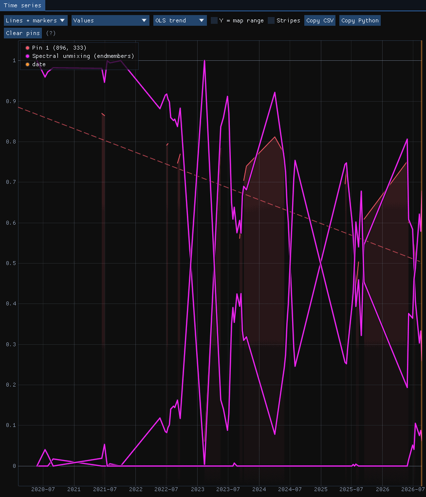
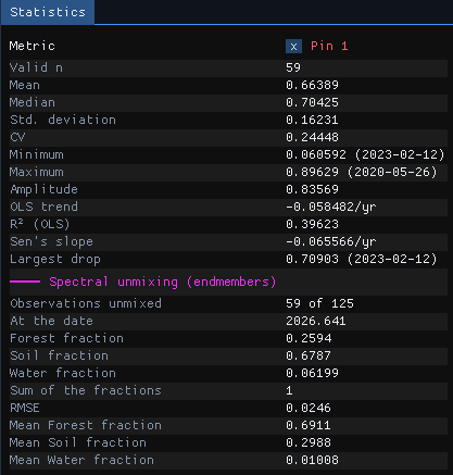
The chart of the pixel at (896, 333): the NDVI and, in magenta, the three fractions over 2020-2026: one fraction near 1 until 2022, falling through 2022 and dropping to 0 in 2023, then swinging between about 0.1 and 0.9 against a second fraction that mirrors it; the third stays near 0. — **The fractions of one pixel**, 2020–2026: forest near 1, then the clearing.

The Statistics table: observations unmixed 59 of 125; at the date 2026.641: forest fraction 0.2594, soil 0.6787, water 0.06199, sum of the fractions 1, RMSE 0.0246; mean forest fraction 0.6911, mean soil 0.2988, mean water 0.01008. — Its numbers at 23 August 2026, and the means.

59 of the 125 dates have a clear observation at this pixel. Until 2022 the forest fraction stays near 1; it falls through 2022 and drops to 0 in early 2023, when the soil fraction takes its place. From then on the two swing against each other with the seasons: a green pasture in the rainy season looks like the forest endmember to a model of three, and a dry one like soil. On 23 August 2026 the pixel is 26% forest, 68% soil and 6% water, rebuilt with an RMSE of 0.025 reflectance.

The three fractions are drawn in the tool's colour; the Statistics table names them and gives the values at the observation nearest the date shown (At the date), their sum and the means over all the observations.

A missing endmember

The swing of the pasture is the model's limit, not noise: dry grass is neither forest nor bare soil. An endmember of dry vegetation (non-photosynthetic vegetation), taken from a pasture in the dry season, would take that share and lower the RMSE there.

06Running it on the series

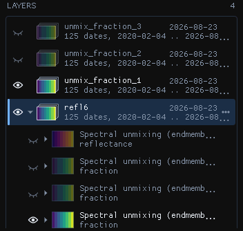
Under Run on the raster, Whole image and Run: the 2.8 million pixels × 125 dates took 130 seconds. The run writes each fraction as a series, a GeoTIFF of one band per date (Int16, scale 0.0001), opened as a new layer that any other tool can take, and four maps, layers of their own:

The Layers panel: three new series unmix_fraction_1 to 3 of 125 dates each, the forest one shown; under refl6, the results: the mean RMSE (reflectance) and the three mean fractions. — **The outputs**: three fraction series, and the maps under the series.

Output	What it holds
Fraction series	Each endmember's fraction at each date (no data where the date had none).
Mean fraction	Each endmember's mean over the dates.
Mean RMSE	The mean error of the rebuilt spectra.
Observations unmixed	How many dates each pixel had.

The forest fraction on 23 August 2026 over the whole image, 0 in dark purple to 1 in yellow: forest blocks and strips along the streams in yellow, pastures in blue and green, the rivers dark. — **Forest fraction**, 23 August 2026.

The soil fraction on the same date: dark over the forest, green and yellow over the pastures, bright yellow over a block of bare fields near the top. — **Soil fraction**, the same date: the cleared fields stand out.

The mean RMSE from 0.007 to 0.042 reflectance: low over the forest and the water, high over many pastures. — **Mean RMSE**, 0.007 to 0.042: low on the forest and the water, high on the pastures the three endmembers describe worst.

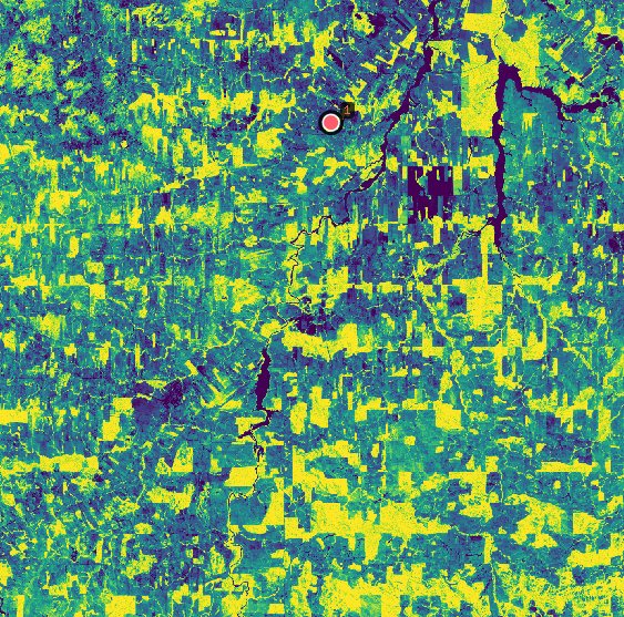
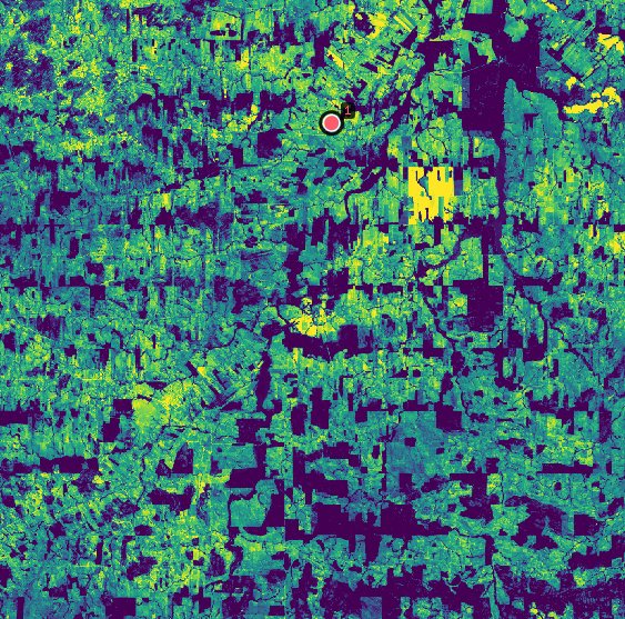
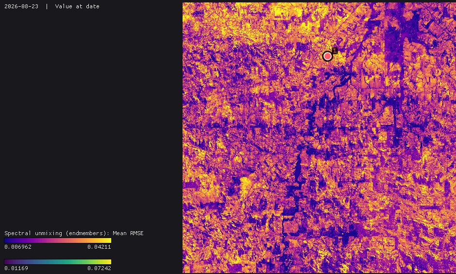
The fraction series are series like any other: open LandTrendr or BFAST on the forest fraction to date the clearings, or the soil fraction to find when fields were bare. They are large (a few hundred MB each here): run on the Visible area or an ROI while choosing the endmembers.

07The constraints

Constraints	Fractions	When
Non-negative, summing to one (FCLS)	0 to 1, adding up to 1	The default: shares of the pixel.
Non-negative (NNLS)	0 or more, any sum	When brightness varies (illumination, slopes) and the sum should follow it.
Summing to one	Any sign, adding up to 1	To see where the endmembers fail: negative fractions and fractions above 1 point at materials not in the list.
None (least squares)	Any	The plain linear model, for comparison.

Without the constraints the fractions can be negative or above one where the endmembers do not describe the pixel; the RMSE shows where.

08A hyperspectral scene

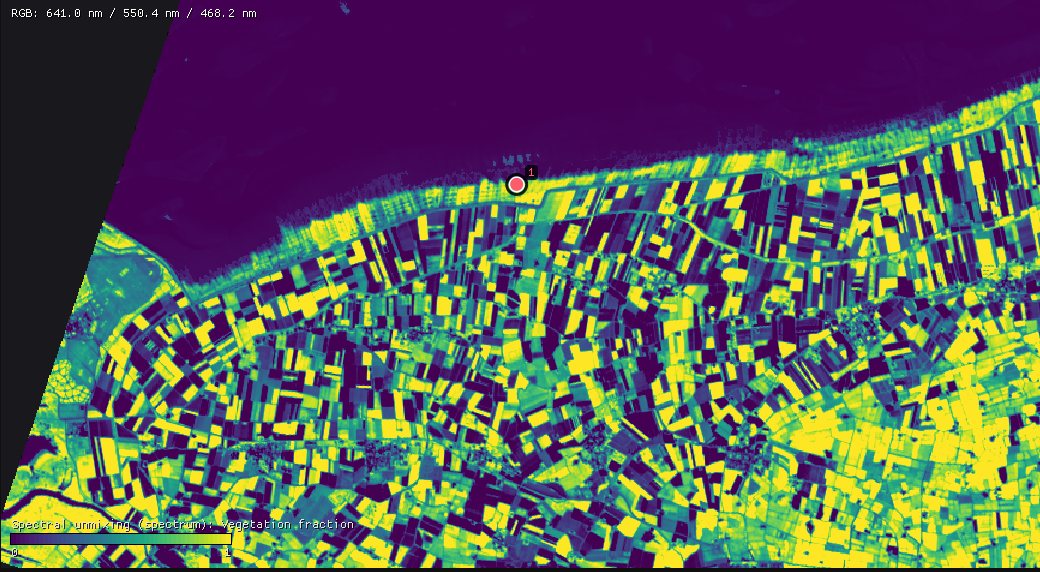
An EnMAP scene (L2A, surface reflectance) of 10 August 2022 on the coast of Groningen, the Netherlands: 1335 × 1288 pixels of 30 m, 224 bands from 418 to 2446 nm. Janus opens the file as it is, as a spectrum, a series whose axis is the wavelength, and the chart draws each pixel's spectrum. Tools → Spectral analysis → Spectral unmixing (spectrum) takes pins' spectra as endmembers, the same way: here a green crop (vegetation), a bare field (soil) and the Wadden Sea (water).

Bands without data

EnMAP's L2A product leaves six bands, 1331 to 1391 nm in the water vapour absorption, without data in every pixel. The endmembers have no value there either, and the tool leaves those bands out on its own: the pixels are unmixed on the other 218, and the rebuilt spectrum breaks at the gap. Nothing to prepare.

The Spectral unmixing (spectrum) window: FCLS; three endmembers, Vegetation, Soil and Water, from pins 1, 2 and 3 with 224 bands each; Add an endmember from...; Run on the raster: whole image. — **The endmembers**: three pins' spectra.

The Statistics table of pin 4 at (443, 677): 218 valid values; vegetation fraction 0.4225, soil 0.2187, water 0.3588, sum 1, RMSE 0.006587. — A mixed pixel: 42% vegetation, 22% soil, 36% water.

The chart of the pixel at (443, 677) against wavelength: its spectrum in green, low in the visible, a red edge near 700 nm, a plateau near 0.24 in the near infrared and two humps in the shortwave infrared; the rebuilt spectrum in magenta follows it closely and breaks, like it, at the bands without data near 1.4 µm; three dashed magenta curves, each endmember's part. — **The spectrum and its rebuild**: the pixel (green), the spectrum the fractions rebuild (magenta) and each endmember's part of it, its spectrum times its fraction (dashed).

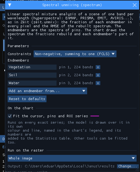
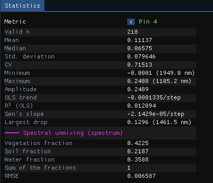
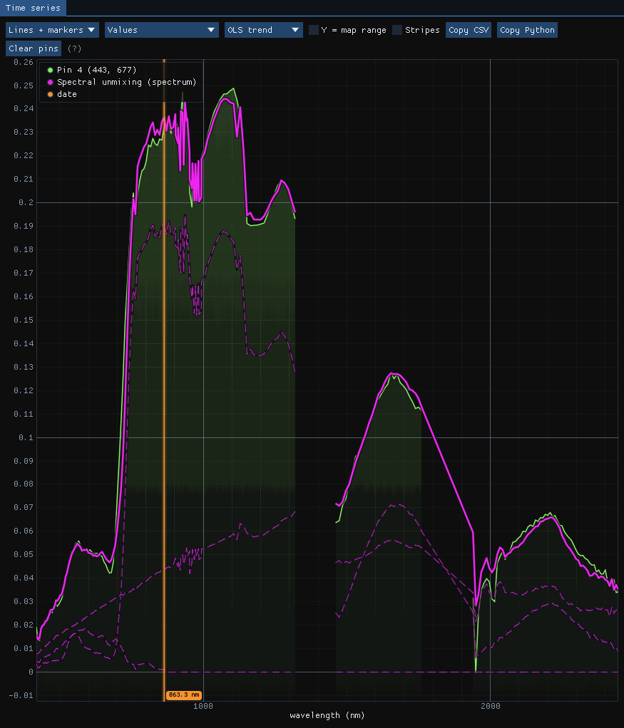
The rebuilt spectrum follows the pixel's over the whole range, with an RMSE of 0.0066 reflectance. The water endmember is nearly black beyond the visible, so on land it acts as shade: it takes the darkness of the pixel (wet soil, shadows, ditches) rather than standing water. Name it so when reading the maps.

Run on the whole scene, the tool took 9 seconds for its 1.7 million pixels of 218 bands. Each fraction and the RMSE are maps in the Layers panel, layers of their own:

The vegetation fraction over the coast, 0 in purple to 1 in yellow: the sea and the mudflats at 0, the fields a patchwork of yellow (green crops) and purple (bare or harvested), the grassland of the south in green and yellow. — **Vegetation fraction**: green crops in yellow, harvested and bare fields in purple.

The RMSE from 0.001 to 0.121 reflectance: low over the sea and many fields, high in yellow over a set of fields scattered over the farmland. — **RMSE**: the bright fields are a cover none of the three endmembers describes. Drop a pin on one, look at its spectrum, and add it as an endmember.

09Against RStoolbox

Zeit's solver against mesma of the R package RStoolbox, with its NNLS solver, on pixels mixed from 4 endmembers in 6 bands (Zeit's own benchmark, benchmarks/vs_originals/unmix.py):

Pixels	RStoolbox	Zeit, 1 thread	Zeit, 19 threads	Agreement
200 × 200	0.84 s	47 ms (18×)	5.4 ms (157×)	fractions to 4e-4
1000 × 1000	21.8 s	1.25 s (17×)	132 ms (165×)	fractions to 4e-4

mesma's NNLS stops at a tolerance, while Zeit solves each pixel exactly: the fractions agree to 4e-4 and Zeit's RMSE is never larger.

10What next

Date the change: LandTrendr or BFAST on a fraction series.
Forest degradation: Tools → Spectral analysis → NDFI (spectral unmixing) unmixes Landsat with the fixed endmembers of Souza et al. (GV, NPV, soil, shade, cloud) into the NDFI, the index CODED uses for logging and fire.
Validate it: classify the fractions and check the map with the Validation guide.
Script it: the same unmixing is zeit.unmix in Python.

11References

Adams, J. B., Sabol, D. E., Kapos, V., Almeida Filho, R., Roberts, D. A., Smith, M. O., Gillespie, A. R. (1995). Classification of multispectral images based on fractions of endmembers: application to land-cover change in the Brazilian Amazon. Remote Sensing of Environment, 52(2), 137–154.
Heinz, D. C., Chang, C.-I. (2001). Fully constrained least squares linear spectral mixture analysis method for material quantification in hyperspectral imagery. IEEE Transactions on Geoscience and Remote Sensing, 39(3), 529–545.
Souza, C. M., Roberts, D. A., Cochrane, M. A. (2005). Combining spectral and spatial information to map canopy damage from selective logging and forest fires. Remote Sensing of Environment, 98(2–3), 329–343.
Guanter, L., et al. (2015). The EnMAP spaceborne imaging spectroscopy mission for Earth observation. Remote Sensing, 7(7), 8830–8857.
Leutner, B., Horning, N., Schwalb-Willmann, J. RStoolbox: remote sensing data analysis in R.
Zeit: the library behind the tools of Janus.

Spectral unmixing, step by step.