Emerging hot spots

01The idea

Emerging hot spot analysis is ESRI's Space Time Pattern Mining tool, also available in R as sfdep's emerging_hotspot_analysis. It has two steps.

First, at every date, it computes the Getis-Ord Gi* of each pixel (Getis & Ord 1992). This statistic sums the values in the pixel's neighbourhood (the pixel included) and compares the sum with what the date's mean would give, as a z-score. A significantly positive Gi* makes the pixel a hot spot at that date, and a significantly negative one makes it a cold spot. The neighbourhood is the pixels within a radius, at that date and at the dates before it.

Second, each pixel's series of Gi* gets a Mann-Kendall trend test. Its dates as a hot or cold spot and its trend then give its pattern, as ESRI defines them.

Gi*: A z-score: how far the sum of a neighbourhood is from what the date's mean would give it. Beyond ±1.96 it is significant at 0.05.
Hot / cold spot: A date at which the pixel's Gi* is significantly positive / negative.
Trend of the Gi*: Whether the pixel's Gi* rises or falls over the dates (Mann-Kendall), which separates intensifying hot spots from diminishing ones.
Pattern: The pixel's history, summed up in one of 17 classes: no pattern, or one of eight kinds of hot spot and the same eight of cold spot.

The values can be anything that varies in space and time: an index, a loss, an anomaly, a count. The analysis needs the whole map (each pixel's neighbourhood), so it runs on the raster only, not on the chart.

02The example

The data of the LandTrendr guide: forty years of NDVI (× 10000), one composite a year from 1985 to 2024, over a circle of about 50 km in central Rondônia, Brazil. This is a forest frontier opened along roads and mostly cleared between 2000 and 2005. The stack is one GeoTIFF with a band per year, opened through a VRT that declares 0 (outside the circle) as no data. It covers 1686 × 1671 pixels of 30 m.

In NDVI, the forest is high and pasture is low, so the hot spots are clusters of forest and the cold spots are clusters of cleared land. The patterns tell how each one changed.

03Opening the tool

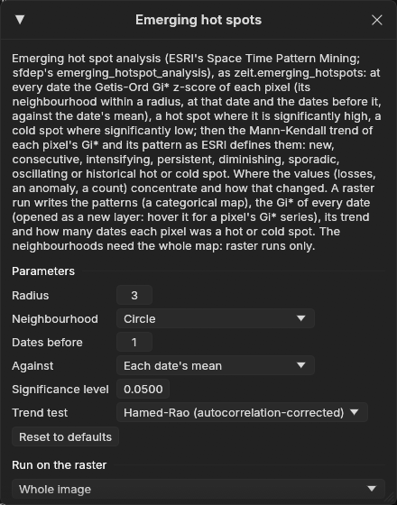
The Emerging hot spots window: its description, the parameters radius 3, neighbourhood circle, dates before 1, against each date's mean, significance level 0.05, trend test Hamed-Rao, and Run on the raster with Whole image. — **The window**, with the radius and neighbourhood used in this guide.

Tools → Spatial pattern analysis → Emerging hot spots, among the trend tools. The tool needs at least three dates, and comes from Zeit, which is built into Janus.

04The parameters

Parameter	Default	What it does
Radius	1 px	The neighbourhood: the pixels within this distance, the pixel included. With 1 and a square these are its 8 neighbours (queen contiguity, sfdep's default). A wider radius finds wider clusters.
Neighbourhood	square	Square: (2 × radius + 1)² pixels. Circle: the pixels whose centres are within the radius.
Dates before	1	The earlier dates also in each date's neighbourhood (sfdep's `k`, ESRI's neighbourhood time step). With 1, each Gi* is smoothed with the date before it.
Against	each date's mean	Each date's mean (as sfdep): a place is hot compared with the others at that date. The whole series' mean: every date is compared with all of them, so a date that is high everywhere is hot everywhere.
Significance level	0.05	A Gi* is a hot or cold spot when its two-sided p-value is below this. The same level applies to its trend.
Trend test	Hamed-Rao	The test of each pixel's Gi* series. Consecutive dates share neighbours, so the series is autocorrelated, and Hamed-Rao corrects for that. Also: the original Mann-Kendall (ESRI's and sfdep's) and Yue-Wang.

At 30 m, the default radius of 1 px measures clusters of 3 × 3 pixels, and the map comes out speckled by single fields. This guide uses a radius of 3 in a circle (pixels within 90 m) and keeps the other defaults.

05Running it

Under Run on the raster, choose the Whole image, the Visible area or the ROI, then Run. The run holds the values of the whole window in memory, along with their Gi*: about 40 bytes per value. If that would exceed 6 GB, Janus refuses and asks for a smaller area. Here the whole image, 40 dates of 2.8 million pixels, takes 4.2 GB, and it ran in 14 s, much of it spent reading the stack.

The Tasks panel: Emerging hot spots on the whole image, 1686 by 1671 pixels, done 100 percent in 14 seconds. — **Tasks**: the whole image in 14 s.

The outputs are GeoTIFFs in %LOCALAPPDATA%\Janus\results by default, opened as layers:

Output	Meaning
Pattern	A class map of the 17 patterns, in the Hotspots colours. It is the layer shown after the run.
Gi* z-score	The Gi* of every date, as a new series layer, opened hidden under the patterns.
Trend of the Gi* (z)	The z of the trend test: positive where the Gi* rises.
Dates a hot spot	How many dates the pixel was a significant hot spot.
Dates a cold spot	The same for cold spots.

06The patterns

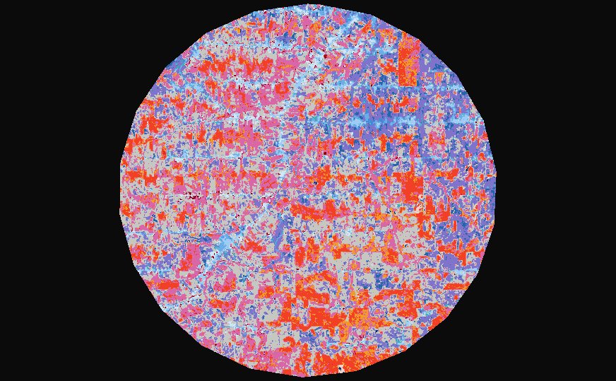
The pattern map over the whole circle: red for intensifying hot spots on the forest blocks, pink for oscillating hot spots, purple for oscillating cold spots on the cleared land, grey for no pattern. — **The patterns** over the whole circle (radius 3, circle, each date's mean).

Each pattern is tested on the hot dates first, then on the cold ones. The cold-spot patterns read the same way as the hot ones, with cold dates instead of hot dates. The last two columns give each pattern's share of the circle in this run.

Pattern	Definition (hot; cold alike)	Hot	Cold
New	Hot at the last date, and only then.	0.4%	0.1%
Consecutive	Hot dates in a single run that reaches the last date, fewer than 90% of them.	0.2%	2.7%
Intensifying	Hot on 90% of the dates or more, the last one included, with the Gi* rising significantly.	11.5%	0.2%
Persistent	The same, without a significant trend.	0.7%	2.7%
Diminishing	The same, with the Gi* falling significantly.	0.0%	2.4%
Sporadic	Hot at the last date, hot on and off before, never cold.	6.2%	1.0%
Oscillating	Hot at the last date, hot on and off before, cold at some earlier date.	21.9%	16.9%
Historical	Hot on 90% of the dates or more, but not at the last.	0.3%	2.0%
No pattern	None of the above.	30.7%

Everything depends on the last date. A pixel that was a cold spot for twenty years but not in 2024 has no pattern (unless it was cold on 90% of the dates, which makes it historical). Against each date's mean, the forest left standing becomes more distinct as the land around it is cleared. Its Gi* rises, so the large forest blocks are intensifying hot spots (red). The cleared land is mostly oscillating cold (purple): it was hot while it was forest, and cold since, with some years in between when it was not significantly cold.

07Reading a pixel

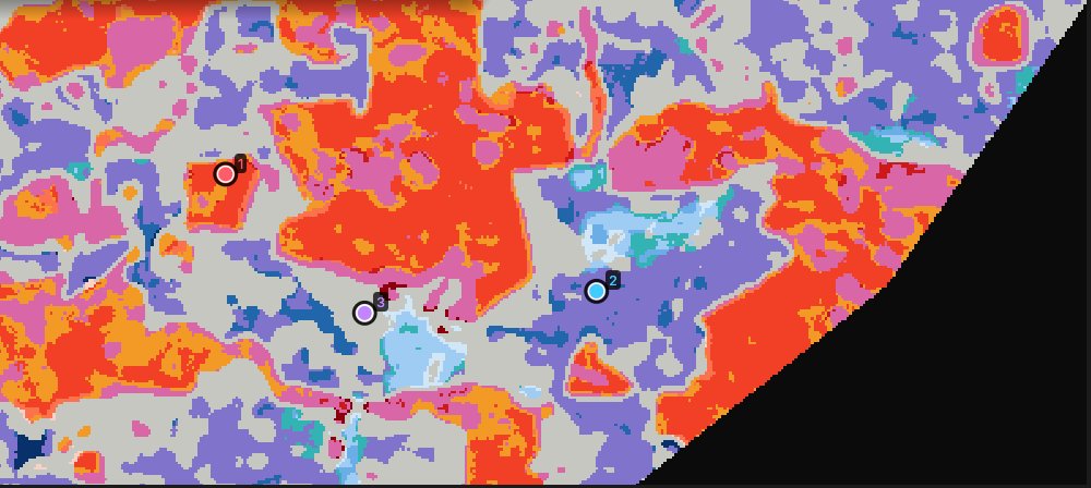
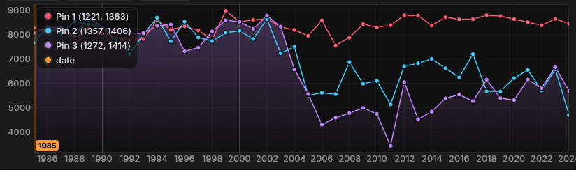
A zoom on the pattern map south-east of the centre, with three pins: pin 1 on a red forest block, pin 2 on purple cleared land, pin 3 on grey. — **Three pins** on the patterns: 1, a forest block; 2 and 3, land cleared in 2005.

The NDVI of the three pins from 1985 to 2024: pin 1 stays near 8500, pins 2 and 3 fall from about 8000 to 4000-6000 in 2004-2005 and stay lower. — **Their NDVI**: pin 1 forest throughout; pins 2 and 3 cleared in 2004–2005.

The patterns come from the Gi* series. The Gi* layer opens hidden under the patterns. Tick its eye in the Layers panel and the chart shows each pin's Gi* series:

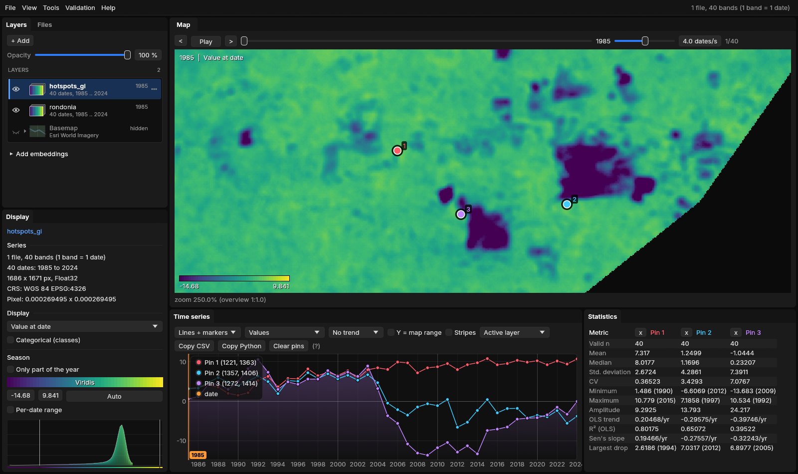
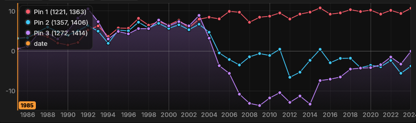
The Janus window with the hotspots_gi layer shown: the Gi* of 1985 on the map, low in the clearings already open, and the Gi* series of the three pins on the chart. — **The Gi* layer**, here at 1985: the dark patches are the clearings already open then.

The Gi* of the three pins: pin 1 rises from about 3 to 10; pins 2 and 3 are between 2 and 9 until 2004, then fall below zero, pin 3 to -13 by 2008 and back to about 0 in 2024, pin 2 between about 0 and -7. — **The Gi* series.** Above 1.96, a hot spot; below −1.96, a cold spot.

Pin 1 (1221, 1363) is a hot spot on 39 of the 40 dates, and its Gi* rises from about 3 to 10 (trend z 6.7): an intensifying hot spot.
Pin 2 (1357, 1406) is a hot spot in 19 of the years up to 2004 and a cold spot at the end, but its cold years are broken by years near the date's mean (2008–2011, 2015, 2017–2018): an oscillating cold spot.
Pin 3 (1272, 1414) is a hot spot for 18 years and a cold spot for 18, from 2005 to 2021 and in 2023. In 2024 its Gi* is −0.1: with its NDVI back to 0.57, it is no longer significantly below that year's mean. Not cold at the last date, and not cold on 90% of the dates: no pattern.

08Against the whole series

Against each date's mean, a place is only hot or cold compared with the rest of the map at that date. As the frontier opened, the mean NDVI fell, so the bar for a cold spot fell with it. Against: The whole series' mean uses one mean and one deviation for all forty years instead. The forest of 1985 is then hot everywhere, and the land cleared since is cold for good:

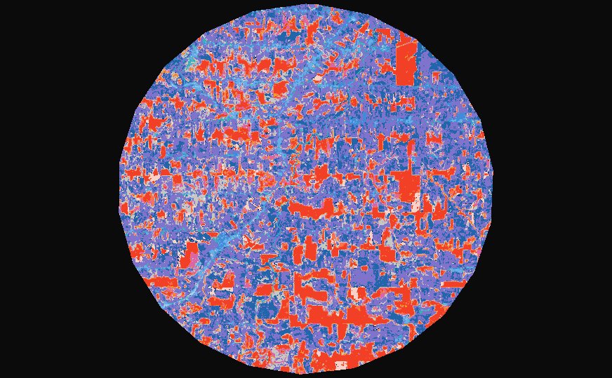
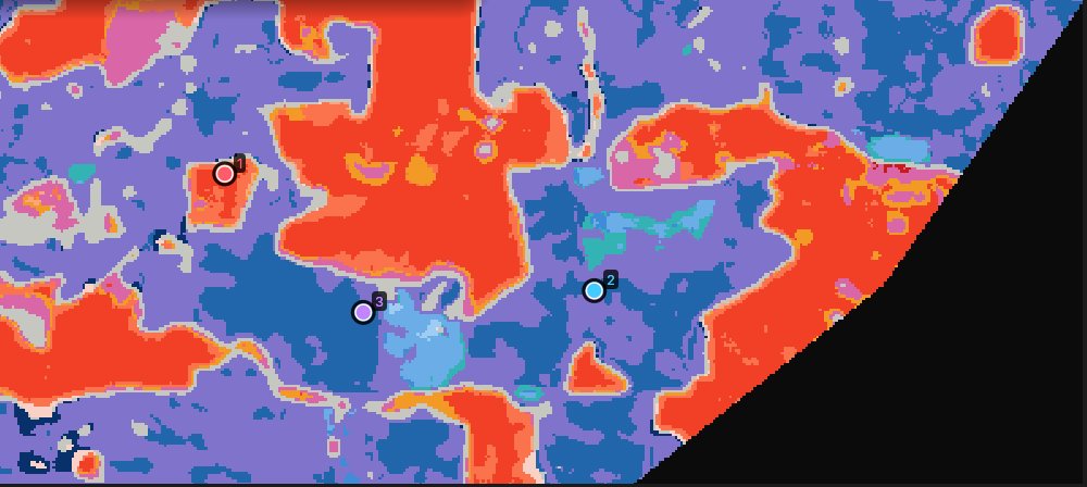
The pattern map against the whole series' mean over the circle: red forest blocks, the rest in purple and blue. — **The whole circle**, against the whole series.

The same zoom as before against the whole series' mean: pin 1 on red, pins 2 and 3 on purple and dark blue. — **The same three pins.**

The cold spots now cover most of the circle: oscillating cold 37.3% and consecutive cold 15.8% (dark blue). The intensifying and persistent hot spots (15.2% and 4.3%) are the forest that still stands. Pin 3 becomes a consecutive cold spot: cold every year from 2005 to 2024, in one run. Pin 2 stays oscillating, because its Gi* of 2009 (−1.7) breaks the run. Pin 1 is still intensifying, hot at every date.

Which to choose

Each date's mean asks where values cluster compared with the rest of the map at that date, which is sfdep's question. The whole series' mean asks where they cluster compared with the whole period, so a change that affects everything shows up everywhere. With a lag (dates before), the Gi* of a date also counts earlier dates against that date's mean, so a rise everywhere lowers it.

The Gi* equals R sfdep's (0.2.5, queen neighbours, k the lag) to 1e-14, and the trend test equals Kendall's to its single precision. The patterns follow ESRI's definitions with the normal p-values of the Gi*. sfdep's differ: it takes each Gi*'s significance from 199 permutations and has rules of its own. On a grid of 50 × 50 cells and 12 dates, sfdep takes 13 minutes (28 s with 9 permutations); Zeit takes 4 to 7 ms.

09What next

Hot spots of change, not of state. Run the analysis on a series of yearly losses (the drop of the index from one year to the next) or of anomalies, to find where the changes themselves concentrate.
Test a region's trend. The trend test guide asks whether a whole region is trending, taking the spatial correlation of its pixels into account.
The events behind the patterns: LandTrendr on the same series maps the year and magnitude of each clearing.
Script it. The same analysis is zeit.emerging_hotspots in Python.

10References

Getis, A., Ord, J. K. (1992). The analysis of spatial association by use of distance statistics. Geographical Analysis, 24(3), 189–206.
Ord, J. K., Getis, A. (1995). Local spatial autocorrelation statistics: distributional issues and an application. Geographical Analysis, 27(4), 286–306.
Esri. How Emerging Hot Spot Analysis works. ArcGIS Pro documentation, Space Time Pattern Mining toolbox.
Hamed, K. H., Rao, A. R. (1998). A modified Mann-Kendall trend test for autocorrelated data. Journal of Hydrology, 204, 182–196.
Parry, J., Locke, D. sfdep: Spatial Dependence for Simple Features. R package.
Zeit: the change detection library behind the tools of Janus.

Emerging hot spots, step by step.