Core Concepts¶

A few conventions run through the whole library. Learn them once and every tutorial and API page will read the same way. If something in Zeit surprises you, the answer is most likely on this page.

Images become time series¶

A satellite revisits the same place again and again. Stack the images of one area in date order and you get a data cube with three axes: time, rows and columns. Now read the cube along its time axis at a single pixel, and you have that pixel's time series: how its reflectance (or a vegetation index such as NDVI) evolved.

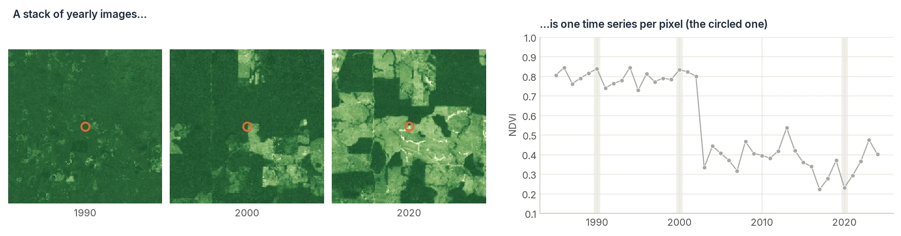
Three yearly NDVI images of the same area and the time series of one pixel — Real Landsat NDVI over Rondônia, Brazil. The circled pixel stays at about 0.8 while it is forest, then drops to 0.3–0.5 after being cleared in 2003. *Data: annual Landsat NDVI composites exported from LT-GEE on Google Earth Engine.*

Nearly every algorithm in Zeit works one pixel at a time. It reads a pixel's time series, fits a model to it, and returns a few numbers (a break date, a trend slope, a class). Run over every pixel, those numbers become maps. Because pixels are independent, the work splits cleanly across CPU cores and across machines.

Array shapes¶

What	Shape	Notes
A single pixel	`(time,)`	1-D NumPy array or list.
A single-band cube	`(time, rows, cols)`	The default input for almost everything. `zeit.load_raster` reads a GeoTIFF with one band per date into this shape, with the dates in a `time` coordinate and the georeferencing in `.rio`.
A multi-band cube	`(time, band, rows, cols)`	What `build_time_series` returns (as an xarray `DataArray`), and what `zeit.ccdc` takes.
Per-pixel results	`xarray.Dataset` of `(rows, cols)` maps	One variable per output, with the cube's coordinates and CRS: `result.slope`, `result["TRS5.sos"]`. Outputs with several values per pixel add a leading dim, such as `(vertex, y, x)` or `(year, y, x)`.

An exception

The deep-learning models follow PyTorch conventions (for example (batch, channels, time) for TempCNN). Their pages say so explicitly.

Dates: each family has its own convention¶

This is the single most common source of confusion, because each algorithm keeps the time convention of the software it was ported from:

Algorithm	What you pass	Example
LandTrendr	Nothing for a cube with dates (read from its `time` coordinate); integer years for a numpy array or a single series	`years=np.arange(1985, 2025)`
CCDC	Nothing for a cube with dates (read from its `time` coordinate); any dates for a numpy array or an unnamed stack	`dates=["2020-01-15", "2020-01-31", ...]`
Tmask	Python ordinal days (`date.toordinal()`)	`date(2020, 7, 1).toordinal()` → `737607`
BFAST, BFAST Monitor, BFAST Lite	Nothing for a cube with dates: the regular series of R's `ts`, `start_time` (fractional year) and `frequency` (observations per year), is read from them. Both for a series without dates.	`start_time=2010.0, frequency=23` for 16-day composites
Mann-Kendall	Nothing. The slope is per time step, so use one value per year for a per-year slope (or `method="seasonal"`).
Phenology	Nothing for a cube with dates (read from its `time` coordinate); any dates for a numpy array or a single series	`dates=pd.date_range("2019-01-01", periods=69, freq="16D")`
TWDTW	Nothing for a cube with dates (read from its `time` coordinate); patterns are series indexed by dates, matched by day of year around the year	`pd.Series(values, pd.date_range("2021-01-01", periods=23, freq="16D"))`
SNIC, SOM	Nothing. Time is just another feature.

Converting from pandas / xarray timestamps:

import pandas as pd

t = pd.to_datetime(cube.time.values)

years    = t.year.values                                   # LandTrendr (numpy input)
ordinals = [d.toordinal() for d in t.date]                 # Tmask

Values and scale factors¶

Most surface-reflectance and index products are stored as integers scaled by 10,000 (so NDVI 0.73 is stored as 7300). Zeit keeps each reference algorithm's own assumptions:

CCDC and Tmask expect reflectance × 10,000. Their thresholds (the lasso penalty, the cloud tests) are defined on that scale. Pass 0–1 floats and results will be wrong. Tmask has a scale_factor argument if your data is already 0–1.
LandTrendr works on any scale, but min_magnitude in extract_events is in the same units as your data (1500 for NDVI × 10,000, 0.15 for plain NDVI).
Trend, BFAST and phenology work on any scale. Slopes and magnitudes come back in the units you put in.

Missing data¶

Use NaN for missing observations in float arrays. Most algorithms skip NaNs per pixel.
zeit.landtrendr, zeit.ccdc, the BFAST family, zeit.mann_kendall and zeit.phenology also leave out the raster's NoData value and, for integer data without one, 0 (how Earth Engine exports masked pixels). Set nodata= to another value, or nodata=None to treat only NaN as missing.
CCDC uses its own QA codes (Fmask convention: 0 clear, 1 water, 2 shadow, 3 snow, 4 cloud, 255 fill). See CCDC.

Ways to call an algorithm¶

The change-detection, trend and phenology algorithms each have a single entry point for every form of data. zeit.landtrendr, zeit.ccdc, zeit.bfast_monitor, zeit.bfast_lite, zeit.bfast, zeit.mann_kendall and zeit.phenology read what they are given and return the same xarray.Dataset (of vertices, segments or metrics), georeferenced when the input is:

flowchart LR
    A["One pixel's series"] --> L["<code>zeit.landtrendr(data)</code><br/><code>zeit.ccdc(data)</code><br/><code>zeit.bfast_monitor(data, ...)</code><br/>…"]
    B["NumPy array or cube in memory"] --> L
    C["GeoTIFF bigger than RAM<br/>(read lazily, block by block)"] --> L
    D["Xarray / Dask cube"] --> L
    L --> E["xarray.Dataset"]

Data	Use it when	Example
One pixel	Exploring, plotting, testing parameters on a few series	`zeit.landtrendr(values, years=years)`, `zeit.ccdc(df)`, `zeit.mann_kendall(values)`
Array or cube	The data fits in memory	`zeit.landtrendr(cube)`, `zeit.ccdc(cube, qa="fmask")`, `zeit.phenology(cube)`
Raster file	A GeoTIFF too big for memory. It is read and computed in blocks.	`zeit.landtrendr("stack.tif", chunks="auto")`, `zeit.bfast_monitor("ndvi_16d.tif", "2022-01-01", chunks="auto")`
Dask cube	Lazy cubes (STAC, Zarr), clusters, cloud storage	`zeit.landtrendr(cube)`, `cube.zeit.ccdc()`, `cube.zeit.bfast_lite()`
CLI	Scripts, cron jobs and HPC schedulers, no Python needed	`zeit landtrendr ...`, `zeit ccdc ...`, `zeit bfast-monitor ...`, `zeit mann-kendall ...`

All run the same C++ code; only the way the data is read and the result is computed changes. A dask cube gives a lazy result, computed when you call .compute() or write it with save_raster; in-memory data gives an in-memory result.

Each function also has an accessor form, available on every xarray object once you import zeit: cube.zeit.landtrendr(), cube.zeit.bfast_monitor("2022-01-01"), … See the Xarray accessor reference for the full list of methods.

Parallelism¶

n_jobs controls C++ threads (OpenMP). The default -1 uses all cores but one, so your machine stays responsive. n_jobs=1 runs single-threaded, which is handy for debugging.
Dask splits a cube into spatial chunks and processes them in parallel, on one machine or a cluster. Always keep the time axis in a single chunk (chunks={"time": -1, "y": 512, "x": 512}), because each pixel needs its whole history.
When Dask already runs one task per core, set n_jobs=1 inside each task to avoid oversubscribing the CPU.
On macOS, the pre-built wheels run the C++ core single-threaded. Dask parallelism still works. See Installation to enable OpenMP.

Faithful ports, validated¶

Each algorithm is a port of a specific reference implementation (the original IDL LandTrendr, the MATLAB CCDC, R's bfast, phenofit, sits and so on). Parameters keep their original names and defaults where possible, so published parameter choices carry over. The Benchmarks section documents how each port was compared with its reference, and where it differs on purpose.