TempCNN
(batch, bands, time) tensors with a fixed lengthsits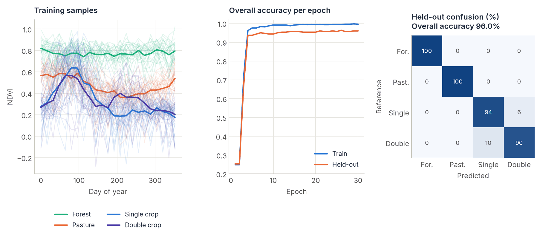
docs/scripts/make_figures.py.TempCNN is a 1D convolutional neural network designed for classifying per-pixel satellite image time series. It's a simpler, faster-to-train alternative to attention-based models like LightTAE, and a strong baseline for most pixel time-series classification tasks. It was introduced in:
Pelletier, C., Webb, G. I., & Petitjean, F. (2019). Temporal convolutional neural network for the classification of satellite image time series. Remote Sensing, 11(5), 523. https://doi.org/10.3390/rs11050523
zeit.ai.TempCNN was ported layer-for-layer from the R package sits's sits_tempcnn() (R/sits_tempcnn.R, R/api_torch.R), so trained weights are directly portable between the two via state_dict() — no name translation needed. This was checked by exporting a trained sits_tempcnn() model's weights, loading them into zeit.ai.TempCNN via load_state_dict(), and confirming the predictions match sits's own output within float32 numerical tolerance on identical input.
How It Works
TempCNN treats the time axis of a pixel's spectral history like the spatial axis of a 1D signal, and applies a stack of 1D convolutions along it:
- Three convolutional blocks (
Conv1d -> BatchNorm1d -> ReLU -> Dropout, default widths(64, 64, 64)and kernel sizes(3, 3, 3)), each convolving over the time axis while keeping every spectral band as a separate input channel. - Flatten: the full
(hidden_dim, n_times)feature map is flattened into a single vector — not global-average-pooled. This is a deliberate architectural choice matchingsits's implementation: it means the dense layer's input size is tied ton_times, so a givenTempCNNinstance is fixed to one sequence length for its lifetime (unlike LightTAE, whose attention mechanism can be more flexible about padding, thoughday_offsetsis still fixed per-instance too). - Dense block (
Linear -> BatchNorm1d -> ReLU -> Dropout, default256nodes) followed by a final linear classifier producingnum_classeslogits (softmax applied externally, e.g. viatorch.nn.functional.cross_entropyor manually at inference time).
When to Use It
| TempCNN | LightTAE | |
|---|---|---|
| Best for | Fast baselines, shorter/noisier series, limited training data | Longer, well-sampled series where attention over specific timesteps helps |
| Compute cost | Lower (no attention, no positional encoding) | Moderate |
| Cross-validated against | sits_tempcnn() (R) |
sits_lighttae() (R) |
See the LTAE & LightTAE tutorial for the attention-based alternative, and the UTAE tutorial if you need whole-patch spatial segmentation rather than per-pixel classification.
From a cube to a map
TempCNN classifies each pixel from its series of bands, (time, band). From a cube and labelled points or polygons:
import zeit
from zeit import ai

cube = zeit.load_raster("s2_ndvi_evi_2022.tif")            # (time, band, y, x)
samples = ai.samples(cube, "samples.gpkg", label="class")   # one sample per pixel
model = ai.train(ai.TempCNN, samples, epochs=50)
classes = ai.predict(model, cube)                           # label (y, x), georeferenced
The flatten before the dense layer ties a model to the number of dates it was built for (as in sits): the cube to classify needs as many, e.g. the same composites of another year. See Deep Learning for the samples, the validation blocks and the normalization.
Instantiating the Model
zeit.ai.train builds the model for you from the samples (bands, dates, classes); the arguments below pass through it, e.g. ai.train(ai.TempCNN, samples, dropout_rates=(0.3, 0.3, 0.3)). To build it yourself:
from zeit.ai import TempCNN

model = TempCNN(
    in_channels=n_bands,
    n_times=n_times,               # fixed sequence length this instance is built for
    num_classes=10,
    hidden_dims=(64, 64, 64),       # widths of the 3 conv blocks
    kernel_sizes=(3, 3, 3),
    dropout_rates=(0.2, 0.2, 0.2),
    dense_layer_nodes=256,
    dense_layer_dropout_rate=0.5,
)

device = torch.device("cuda" if torch.cuda.is_available() else "cpu")
model = model.to(device)
A loop of your own
zeit.ai.train covers the usual case. For anything else (another optimizer, a scheduler, augmentation), the SampleSet is a PyTorch Dataset whose items hold the normalized x, the label y and the date positions; see A loop of your own. A model trained this way can still be classified with zeit.ai.predict after zeit.ai.train(model, samples, epochs=0) records the samples' metadata in it.
Validation Against sits
TempCNN was validated end-to-end against sits_tempcnn(): a model trained in R was exported, its weights loaded into zeit.ai.TempCNN via load_state_dict() (a direct, layer-for-layer match — no key renaming), and run on the same input. Outputs matched sits's predictions within float32 numerical tolerance.
References
- Pelletier, C., Webb, G. I., & Petitjean, F. (2019). Temporal convolutional neural network for the classification of satellite image time series. Remote Sensing, 11(5), 523. https://doi.org/10.3390/rs11050523
- e-sensing/sits: https://github.com/e-sensing/sits