BFAST Monitor

Near-real-time change detection. BFAST Monitor learns what "normal" looks like for each pixel from a stable history period, then checks every new observation against it and reports the first moment the pixel stops behaving normally. This is the logic behind many operational deforestation alert systems.

AnswersIs something changing now, compared with the stable past? Since when?

InputA regular series of one index, e.g. 16-day NDVI composites

OutputBreak date, magnitude and a has-break flag per pixel

ReferenceVerbesselt et al. (2012), R package bfast

What BFAST Monitor produces. A synthetic 16-day NDVI series with 12% missing observations. The model is fitted on the history period (2010–2015) and projected forward. A drop is injected in May 2017 (2017.4). BFAST Monitor flags it at 2017.57, once enough evidence has accumulated to be statistically significant.

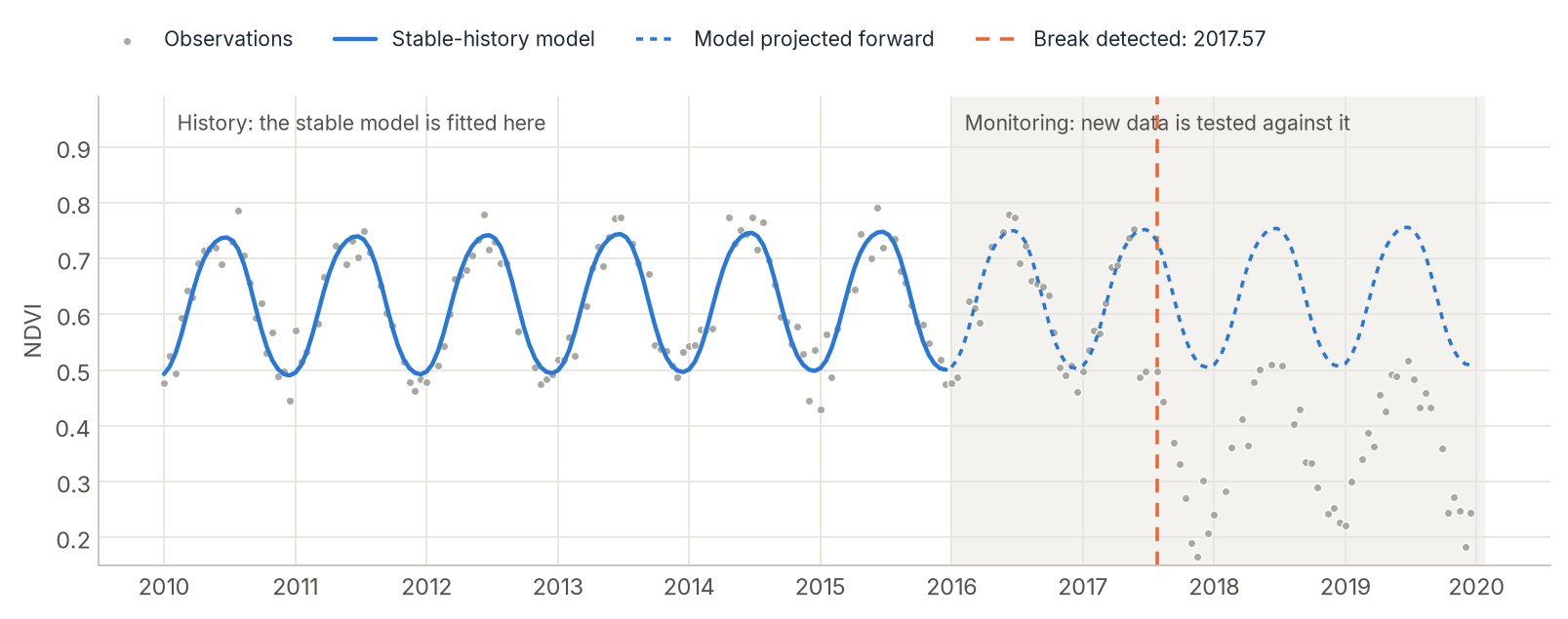
How it works

1. Fit the history. For each pixel, observations before monitor_start are fitted with a regression made of a linear trend plus order seasonal harmonics.
2. Monitor. For each later observation, the residual against that model is computed. A moving sum of residuals (the OLS-MOSUM process) is compared with a boundary that widens over time.
3. Flag. The first time the process crosses the boundary is the detected break. If it never crosses, the pixel is stable.

Because the test accumulates evidence, a single cloudy outlier does not trigger an alarm, but a persistent shift does, usually within a few observations.

Time is regular, not calendar-based

Like R's ts objects, BFAST uses a synthetic, regular time axis: observation i is at start_time + i / frequency. Zeit reads both from the cube's dates (frequency from their median spacing, start_time from the first date), so composite your data to a fixed step first (regularize_time_series) and use NaN for gaps. For a series without dates, give start_time as a whole year (e.g. 2010.0) so the harmonics align with the calendar.

Step by step

1. Prepare a regular series

import zeit

# cube from build_time_series(...), see "STAC Data Cubes"
ndvi = (cube.sel(band="nir") - cube.sel(band="red")) / (cube.sel(band="nir") + cube.sel(band="red"))
ndvi_16d = zeit.regularize_time_series(ndvi, freq="16D", method="median")   # (time, y, x)
ndvi_16d = ndvi_16d.chunk({"time": -1, "y": 256, "x": 256})

16-day composites give frequency=23 observations per year, monthly data frequency=12. Zeit infers it from the dates.

2. Monitor

result = zeit.bfast_monitor(
    ndvi_16d,
    "2022-01-01",               # history before, monitoring from here on (or 2022.0)
    h=0.25,                     # MOSUM window, fraction of the history length
    period=10,
    alpha=0.05,
).compute()                     # a dask cube gives a lazy result
result.attrs["start_time"], result.attrs["frequency"]   # e.g. (2010.0, 23), read from the dates

3. Read the output

The result is an xarray.Dataset with one (y, x) map per metric, on the grid and CRS of the cube:

has_break = result.has_break == 1
break_time = result.breakpoint      # fractional year, NaN if none
magnitude = result.magnitude        # median residual in the monitoring period

Variable	Meaning
breakpoint	Fractional-year time of the first detected break, NaN if none.
breakpoint_idx	0-based index of that observation in the input series.
magnitude	Median residual over the monitoring period: size and direction of the shift. Negative means lower than expected (e.g. vegetation loss on NDVI).
sigma	Residual standard error of the history fit.
n_history	Valid observations used to fit the history.
has_break	1.0 if a break was detected, else 0.0.
valid	0.0 if the history was too short to fit; the other metrics are then NaN.

A typical alert map keeps breaks that also go in the expected direction:

alerts = has_break & (magnitude < -0.1)

Save the maps

zeit.save_raster(result, "results/bfm")        # breakpoint.tif, magnitude.tif, ... georeferenced

Other inputs

The same function takes a raster on disk, a numpy array or a single pixel (all inputs):

# A GeoTIFF larger than memory, with its dates in the band names: read and computed block by block
bfm = zeit.bfast_monitor("ndvi_16d.tif", "2022-01-01", chunks="auto")
zeit.save_raster(bfm, "results/bfm")

# A numpy (time, y, x) array or one pixel's series without dates: give the time axis
bfm = zeit.bfast_monitor(ndvi_numpy, 2022.0, start_time=2010.0, frequency=23)
px = zeit.bfast_monitor(values, 2022.0, start_time=2010.0, frequency=23)

From the shell: zeit bfast-monitor.

Parameters

Parameter	Default	Effect
monitor_start	required	Start of the monitoring period: a date or a fractional year.
start_time	from the dates	Time of the first observation, as a fractional year.
frequency	from the dates	Observations per year.
order	3	Number of seasonal harmonics.
h	0.25	MOSUM window as a fraction of the history. Must be 0.25, 0.5 or 1.0.
period	10	How far ahead, in history lengths, the boundary is valid. Must be 2, 4, 6, 8 or 10.
alpha	0.05	Significance level.
min_valid	10	Minimum valid history observations.

h and period index a table of simulated critical values (from strucchangeRcpp), so other values raise an error instead of being silently extrapolated.

Good practice

Choose a genuinely stable history

This port uses history="all": the whole pre-monitoring period is assumed stable. If that history contains a disturbance, the model is wrong and false alarms follow. In tests on pure noise at alpha=0.05, R's own bfastmonitor(history="all") flagged about 44% of series, and Zeit matched it (about 42%). Pick a disturbance-free history window, require a minimum magnitude, and treat single-pixel detections with caution.

• Use at least 2–3 years of history so the seasonal cycle is well estimated.
• Combine with a spatial filter (for example apply_mmu_filter) to drop isolated alerts.
• For a retrospective analysis of the whole series, use BFAST Lite instead.

Implementation notes and validation

Scope. Only bfastmonitor()'s default monitoring process (type="OLS-MOSUM") with history="all" is ported. R's default history="ROC" (reverse-CUSUM trimming of unstable history) and history="BP" are not. The design matrix matches bfastpp(): response ~ trend + harmon.

Validation. Compared directly with R's bfastmonitor() on six scenarios: a mid-series break, no break, an early break, NaN gaps in the history, monthly data, and non-default h/period. All six matched to floating-point tolerance (identical breakpoint_idx, n_history; differences of 1e-11 to 1e-13 in breakpoint, magnitude, sigma). See Benchmarks.

References

• Verbesselt, J., Zeileis, A., & Herold, M. (2012). Near real-time disturbance detection using satellite image time series. Remote Sensing of Environment, 123, 98–108. doi:10.1016/j.rse.2012.02.022
• Verbesselt, J., Hyndman, R., Zeileis, A., & Culvenor, D. (2010). Phenological change detection while accounting for abrupt and gradual trends in satellite image time series. Remote Sensing of Environment, 114(12), 2970–2980. doi:10.1016/j.rse.2010.08.003
• Chu, C.-S. J., Stinchcombe, M., & White, H. (1996). Monitoring structural change. Econometrica, 64(5), 1045–1065. doi:10.2307/2171955
• Zeileis, A., Leisch, F., Kleiber, C., & Hornik, K. (2005). Monitoring structural change in dynamic econometric models. Journal of Applied Econometrics, 20(1), 99–121. doi:10.1002/jae.776
• R packages bfast and strucchangeRcpp.