Deep Learning

When you have labelled examples, neural networks usually give the most accurate land-cover and change maps. zeit.ai provides PyTorch implementations of the architectures most used for satellite image time series, ported layer for layer from their reference code so that trained weights are interchangeable.

A typical result. A TempCNN trained for 30 epochs on noisy, cloud-contaminated NDVI series of four classes. Forest and pasture are separated perfectly; the remaining errors are between single and double cropping, whose second season is weak in many samples. See the TempCNN tutorial.

Available models

Model	Task	Input	Dedicated Tutorial	Cross-validated against
LTAE & LightTAE	Per-pixel time series classification	(Batch, Time, Bands)	LTAE & LightTAE	sits_lighttae() (R)
TempCNN	Per-pixel time series classification	(Batch, Bands, Time)	TempCNN	sits_tempcnn() (R)
UTAE	Spatio-temporal segmentation (whole-patch class map)	(Batch, Time, Bands, H, W)	UTAE	Official VSainteuf/utae-paps reference (bit-for-bit exact)
Siamese Change Detector	Bi-temporal change detection (two dates)	Two (Batch, Bands, H, W) images	Siamese Change Detector	Independent implementation (not a line-for-line port)
GeoFoundationViT	Transfer learning from pretrained geospatial foundation models	Backbone-dependent	GeoFoundationViT	Inherits correctness from the loaded backbone

Choosing a model:

• Have a long, well-sampled per-pixel time series and want the best accuracy? Try LightTAE first, and TempCNN as a faster/simpler baseline.
• Need a class map over a spatial patch, not just individual pixels? Use UTAE.
• Have exactly two dates and want a change map between them? Use the Siamese Change Detector.
• Have very little labeled data for your task? Consider GeoFoundationViT to transfer-learn from a large pretrained backbone.

From a cube to a map

The models take tensors; zeit.ai takes them from a cube and labelled samples to a georeferenced map in three calls, as train_classifier and classify do for a random forest.

1. Samples

import zeit
from zeit import ai

cube = zeit.load_raster("s2_2022.tif")          # (time, band, y, x), dates in the band names
samples = ai.samples(cube, "samples.gpkg", label="class")
samples                                          # SampleSet(2140 pixels: 1712 train, 428 val; 23 dates x 4 bands; ...)

The samples are points or polygons with a class column, in any CRS. For the pixel models (TempCNN, LightTAE) each sample is one pixel's series, (time, band), and a polygon gives every pixel it covers. For the patch models (UTAE, SiameseChangeDetector, GeoFoundationViT) pass patch= a size in pixels: each sample is the window around a point or a polygon (large polygons are tiled by windows), with every labelled pixel in it. Patch models learn best from polygons: a window around a point has a single labelled pixel.

Two things happen here that are easy to get wrong by hand:

• Validation in spatial blocks. A fifth of the samples is kept for validation (split=0.2), but by whole blocks of 64 × 64 pixels (split_by="block", block_size=64). Neighbouring pixels are nearly the same, so a validation set of pixels drawn at random next to the training ones measures how well the model remembers, not how well it generalizes.
• Normalization. Each band is scaled by its 2% and 98% quantiles in the training samples, as sits does, and the same scaling is applied when predicting. Missing values become 0 after it; fill gaps first (e.g. with zeit.smooth) if clouds are frequent.

2. Train

model = ai.train(ai.TempCNN, samples, epochs=50)
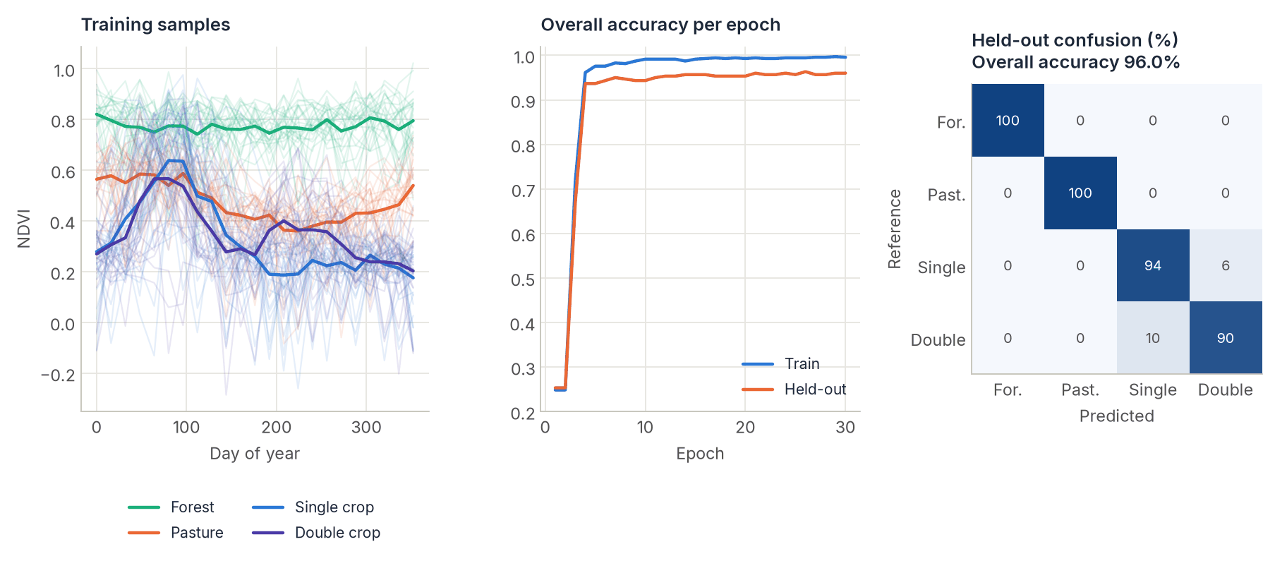
model.zeit_history_[-1]                          # {'epoch': 31, 'train_loss': ..., 'val_loss': ..., 'val_accuracy': 0.94}

train builds the model from its class with the samples' numbers of bands, dates and classes (other arguments of the model pass through, e.g. dropout_rate=0.3), trains it with Adam, stops when the validation loss has not improved for 10 epochs and keeps the best epoch. It runs on the GPU when there is one (device="auto"). loss="focal" helps with imbalanced classes.

3. Predict

classes = ai.predict(model, cube, probability=True)
classes.label.zeit.plot()                         # the class map, with its legend
classes.zeit.save("results/classes")              # label.tif, probability.tif
ai.save(model, "tempcnn_2022.pt")                 # with what predict checks

predict checks the bands (by name) and the dates against the training samples, normalizes the cube as they were and classifies every pixel. zeit.classify(cube, model) does the same. A lazy cube stays lazy and is classified block by block. Patch models slide windows of the training size over the image, overlapping by a quarter (overlap=), and average each pixel's probabilities over the windows, weighted down towards their edges, so the map has no seams.

TempCNN, LightTAE and the Siamese and ViT models are built for the number of dates they were trained on, so the cube to classify needs as many (the same composites of another year, for instance). UTAE takes the positions of the dates at each call and classifies any series.

Model	samples(..., patch=)	Dates when predicting
TempCNN, LightTAE	None (pixels)	as many as in training
UTAE	a multiple of 8 (default U-Net)	any
SiameseChangeDetector	even; the data is a pair (before, after)	a pair
GeoFoundationViT	224 for Prithvi (6 bands)	as in training

For change detection with the Siamese model, the data is a pair of images and the classes are e.g. change and same:

pair = (zeit.load_raster("s2_2021.tif"), zeit.load_raster("s2_2023.tif", like="s2_2021.tif"))
samples = ai.samples(pair, "change_polygons.gpkg", label="class", patch=64)
model = ai.train(ai.SiameseChangeDetector, samples)
change = ai.predict(model, pair)

A loop of your own

The models are ordinary nn.Modules. For a training loop of your own, the SampleSet is a PyTorch Dataset: each item is a dict with x (normalized), y and positions (days since the first date, for the positional encodings):

from torch.utils.data import DataLoader

loader = DataLoader(samples.train, batch_size=64, shuffle=True)
for batch in loader:
    logits = model(batch["x"].permute(0, 2, 1))   # TempCNN takes (batch, band, time)
    ...

To run a model over a whole cube in windows, STACCubeDataset cuts a (lazy) cube into windows that cover it, with the missing values left as NaN and each window's position:

from zeit.ai import STACCubeDataset

dataset = STACCubeDataset(cube, patch_size=64, stride=48)
item = dataset[0]          # {"x": (time, band, 64, 64), "valid", "positions", "row", "col"}

Loss functions for imbalanced classes

Imbalanced classes are very common in change detection and land-cover classification (where the class of interest is often a small minority of pixels). zeit.ai.losses provides three specialized loss functions used throughout the per-model tutorials:

from zeit.ai.losses import FocalLoss, TverskyLoss, ContrastiveSiameseLoss

# Down-weights easy examples, focuses training on hard-to-classify pixels
criterion = FocalLoss(alpha=0.25, gamma=2.0)

# Tunable trade-off between False Positives (alpha) and False Negatives (beta);
# setting beta > alpha penalizes missed changes more than false alarms
criterion = TverskyLoss(alpha=0.3, beta=0.7)

# For metric-learning style training of twin encoders (see the Siamese tutorial)
criterion = ContrastiveSiameseLoss(margin=2.0)

With zeit.ai.train, loss="focal" is the focal loss, ignoring unlabelled pixels; any of these can be passed as loss= too. FocalLoss and TverskyLoss apply to any model's classifier logits ((B, C, H, W) or (B, C) vs. integer labels). ContrastiveSiameseLoss is specific to twin-encoder architectures — see the Siamese Change Detector tutorial.

Next steps

Each architecture has its own tutorial, on how it works, when to use it, its arguments and how it was validated against its reference implementation:

• LTAE & LightTAE
• UTAE
• TempCNN
• Siamese Change Detector
• GeoFoundationViT

---

References

• Garnot, V. S. F., & Landrieu, L. (2021). Panoptic segmentation of satellite image time series with convolutional temporal attention networks. In Proceedings of the IEEE/CVF International Conference on Computer Vision (ICCV) (pp. 4852–4861). https://doi.org/10.1109/ICCV48922.2021.00483
• Garnot, V. S. F., Landrieu, L., Giordano, S., & Chehata, N. (2020). Satellite image time series classification with pixel-set encoders and temporal self-attention. In Proceedings of the IEEE/CVF Conference on Computer Vision and Pattern Recognition (CVPR) (pp. 12322–12331). https://doi.org/10.1109/CVPR42600.2020.01234
• Pelletier, C., Webb, G. I., & Petitjean, F. (2019). Temporal convolutional neural network for the classification of satellite image time series. Remote Sensing, 11(5), 523. https://doi.org/10.3390/rs11050523
• Daudt, R. C., Le Saux, B., & Boulch, A. (2018). Fully convolutional siamese networks for change detection. In 2018 25th IEEE International Conference on Image Processing (ICIP) (pp. 4063–4067). https://doi.org/10.1109/ICIP.2018.8451652
• Jakubik, J., Roy, S., Phillips, C. E., Fraccaro, P., Godwin, D., Zadrozny, B., et al. (2023). Foundation models for generalist geospatial artificial intelligence. arXiv:2310.18660. https://arxiv.org/abs/2310.18660
• Cong, Y., Khanna, S., Meng, C., Liu, P., Rozi, E., He, Y., Burke, M., Lobell, D., & Ermon, S. (2022). SatMAE: Pre-training transformers for temporal and multi-spectral satellite imagery. In Advances in Neural Information Processing Systems 35 (NeurIPS 2022).
• Lin, T.-Y., Goyal, P., Girshick, R., He, K., & Dollár, P. (2017). Focal loss for dense object detection. In 2017 IEEE International Conference on Computer Vision (ICCV) (pp. 2999–3007). https://doi.org/10.1109/ICCV.2017.324
• Salehi, S. S. M., Erdogmus, D., & Gholipour, A. (2017). Tversky loss function for image segmentation using 3D fully convolutional deep networks. In Machine Learning in Medical Imaging (MLMI 2017) (pp. 379–387). https://doi.org/10.1007/978-3-319-67389-9_44