Cloud Masking with Tmask

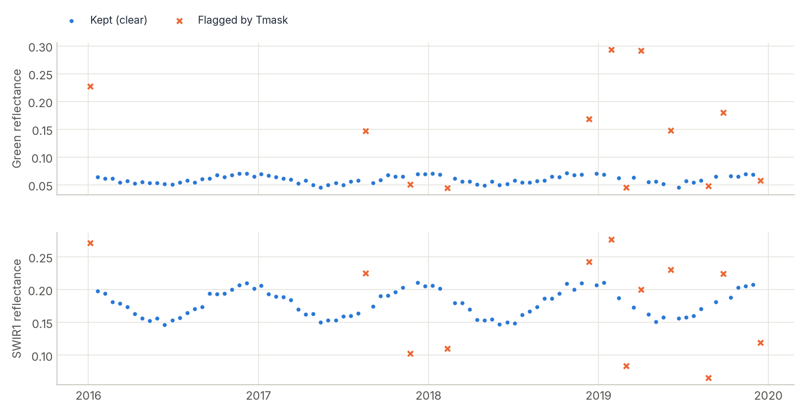
Single-image cloud masks miss thin clouds and small shadows, and every missed cloud looks like a land change to the algorithms downstream. Tmask uses the time dimension instead: it learns each pixel's normal seasonal behaviour and flags observations that are far too bright (cloud) or far too dark (shadow) for that time of year.

AnswersWhich observations are clouds or shadows that the QA band missed?

InputGreen and SWIR1 reflectance stacks (× 10,000) and their dates

OutputA boolean clear mask, same shape as the input

ReferenceZhu & Woodcock (2014)

What Tmask does. Four years of a synthetic 16-day series with 7 clouds (too bright in Green) and 5 shadows (too dark in SWIR1) injected. Tmask fits a robust seasonal model to each band and flags the observations that depart from it too much (orange): all 12 contaminated ones, and nothing else.

How it works

For each pixel, Tmask fits a robust harmonic regression, \(a_0 + c_1 t + a_1 \cos(\omega t) + b_1 \sin(\omega t)\) (iteratively reweighted with Tukey's bisquare, as MATLAB's robustfit in the original and in CCDC's own Tmask, so the outliers barely affect it), to two bands:

• Green, where clouds are much brighter than the land below them;
• SWIR1, where shadows are much darker than expected.

An observation is flagged as cloud when its Green value is more than 0.04 (reflectance) above the seasonal model, and as shadow when its SWIR1 value is more than 0.04 below it. Everything else is kept as clear. The fits run in C++, every pixel in parallel: about 60 µs per pixel of 140 dates on one core, some 190 times faster than the scikit-learn Huber fit used before 0.43 (11 ms per pixel).

Step by step

1. Load Green and SWIR1

Any (time, band, y, x) cube with green and SWIR1 bands, with its dates:

import zeit

cube = zeit.load_raster("landsat/", pattern=r"_(?P<date>\d{8})_(?P<band>\w+)\.tif$")   # reflectance x 10000
cube.band.values      # array(['blue', 'green', 'red', 'nir', 'swir1', 'swir2'], ...)

2. Run Tmask

clear = zeit.tmask(cube, green="green", swir="swir1")
print(clear.dtype, clear.dims)   # bool ('time', 'y', 'x'); True = clear
print(f"{1 - float(clear.mean()):.1%} of observations flagged")

If your reflectance is already in 0–1, pass scale=1.0. Observations without data (NoData, NaN) are not clear. Pixels with 5 or fewer valid observations are not screened, since there is too little data to model the season. A lazy cube (chunks="auto") stays lazy.

3. Use the mask

For CCDC, convert to its QA codes (0 clear, 4 cloud), and combine with the QA band you already have:

import numpy as np
import xarray as xr

tmask_qa = xr.where(clear, 0, 4).astype(np.uint8)
qa = np.maximum(qa_from_qa_pixel, tmask_qa)     # keep the worst of the two

Do not use (~clear).astype(np.uint8) for CCDC

That produces 1 for clouds, and in CCDC's convention 1 means water, which counts as a valid observation. The clouds would be kept.

For everything else, set the flagged observations to NaN before compositing or smoothing:

ndvi_clean = ndvi.where(clear)

To save it, one band per date:

zeit.save_raster(clear.astype(np.uint8), "results/tmask_clear.tif")

Good practice

• Use Tmask as a second pass. Apply the sensor's own QA mask first (Landsat QA_PIXEL, Sentinel-2 SCL, or apply_cloud_mask=True in build_time_series) to remove the obvious clouds, then Tmask to catch what it missed.
• CCDC already includes it. zeit.ccdc runs the original's Tmask screen internally. Running it beforehand is only needed for other algorithms.
• Large areas. Keep the cube lazy (chunks=): zeit.tmask then works block by block, every pixel of a block in parallel.

References

• Zhu, Z., & Woodcock, C. E. (2014). Automated cloud, cloud shadow, and snow detection in multitemporal Landsat data: An algorithm designed specifically for monitoring land cover change. Remote Sensing of Environment, 152, 217–234. doi:10.1016/j.rse.2014.06.012