Quickstart

In five minutes you will build a small image time series, run LandTrendr on every pixel, and get a map of when the vegetation was lost. Nothing is downloaded: the data is generated in the script, so you can see exactly what goes in and what comes out.

You needPython 3.9+ and pip install zeit-cdts

TimeAbout 5 minutes

You will learnThe input shape, one algorithm call, and how to read its output

1. Install

pip install zeit-cdts

Wheels are published for Windows, macOS and Linux, so no C++ compiler is needed. See Installation for GPU support, Docker, and building from source.

2. Make a tiny image time series

Real analyses start from a stack of images: one layer per date. Here we fake one, a 120 × 120 pixel patch of forest observed once a year from 1990 to 2024, with two clearings added:

• a field cleared in 2003 that stays as pasture;
• a patch cleared in 2016 that then starts to regrow.

Values are NDVI (a vegetation index: about 0.85 for dense forest, 0.3 for pasture) multiplied by 10,000, which is how most satellite products store it.

import numpy as np
import zeit

rng = np.random.default_rng(42)
years = np.arange(1990, 2025)                      # 35 annual observations
n_years, rows, cols = len(years), 120, 120

# A forest (NDVI ~0.85) with noise...
stack = 0.85 + rng.normal(0, 0.03, (n_years, rows, cols))
# ...a field cleared in 2003 that stays as pasture,
stack[years >= 2003, 20:60, 15:70] = 0.35 + rng.normal(0, 0.04, (np.sum(years >= 2003), 40, 55))
# ...and a patch cleared in 2016 that starts to regrow.
regrow = np.clip((years - 2016) * 0.06, 0, 0.4)[:, None, None]
after = (years >= 2016)[:, None, None]
stack[:, 70:105, 50:110] = np.where(after, 0.30 + regrow, stack[:, 70:105, 50:110])
stack = (stack * 10000).astype(np.float32)         # NDVI x 10000, like most products

print(stack.shape)   # (35, 120, 120) -> (time, rows, cols)

The one shape to remember

Almost every Zeit function takes an array shaped (time, rows, cols): the first axis is the date, the last two are the image. zeit.load_raster reads a GeoTIFF with one band per year into this shape, with the years in a time coordinate and the georeferencing in .rio.

3. Run LandTrendr on every pixel

LandTrendr simplifies each pixel's history into a few straight segments. The breakpoints between segments, called vertices, mark the moments when something changed.

lt = zeit.landtrendr(stack, years=years)

That one call fits all 14,400 pixels in parallel, in C++. A numpy array has no dates, so years gives the year of each layer. By default (direction="loss") LandTrendr looks for drops in the index, i.e. vegetation loss on NDVI. Use direction="gain" for indices where disturbance makes the value go up.

lt is an xarray.Dataset: the year and fitted value of each vertex (vertex_year, vertex_value), their number (n_vertices) and how well each fit follows its data (rmse).

4. Turn the fit into a map of events

The vertices are compact but not yet a map. extract_events scans each pixel's segments and keeps the largest loss:

loss = zeit.extract_events(lt, min_magnitude=1500)

years_found, n_pixels = np.unique(loss["yod"], return_counts=True)
print({int(y): int(n) for y, n in zip(years_found, n_pixels)})
# {0: 10095, 1990: 2, 1997: 1, 1998: 1, 2001: 1, 2002: 2199, 2015: 2100, 2022: 1}

loss is an xarray.Dataset of 2-D maps, all shaped (rows, cols):

Variable	Meaning
yod	Year of the vertex where the loss begins, i.e. the last year before the drop. 0 means no event.
magnitude	How much the index fell (here in NDVI × 10,000).
duration	How many years the fall took. 1 means abrupt.
pre_val, post_val	Index value before and after the event.
rate	magnitude / duration.
dsnr	magnitude divided by the fit's RMSE: a signal-to-noise ratio.

So the output reads: about 2,200 pixels lost vegetation right after 2002, and about 2,100 right after 2015. Those are the two clearings (2003 and 2016). Only six pixels out of 14,400 were flagged by noise.

yod is the year before the change

LandTrendr places a vertex on the last stable year and the next vertex on the first disturbed one. yod reports the first of the two, so the first year in which the loss is visible is loss["yod"] + 1. Keep this in mind when comparing with LT-GEE, whose change maps report the start vertex year plus one.

5. Look at the result

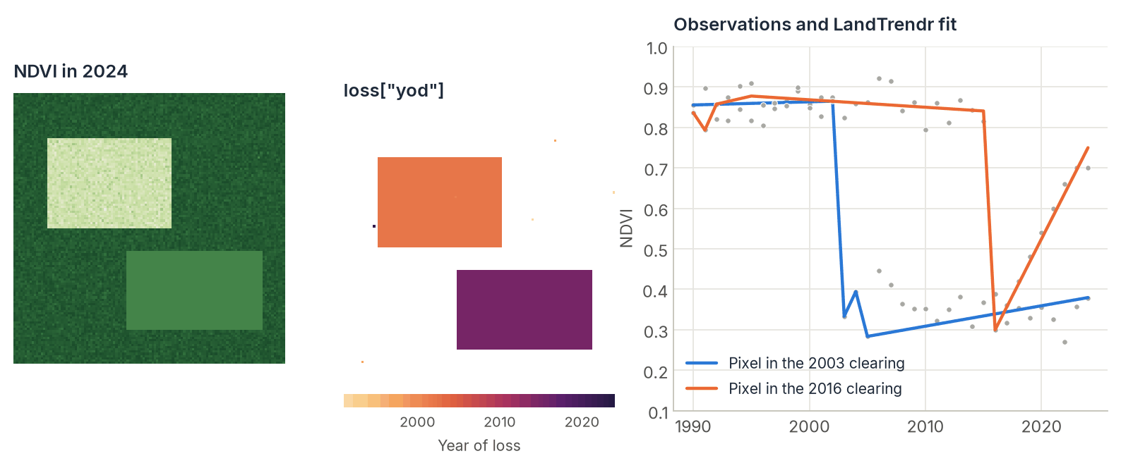
Left: the last image. Middle: the yod map, one color per event year. Right: one pixel from each clearing, with LandTrendr's fitted segments. The 2016 clearing's regrowth shows up as a rising segment after the drop. This figure is produced by the exact code on this page.

To plot it yourself:

import matplotlib.pyplot as plt

yod = (loss["yod"] + 1).where(loss["yod"] > 0)   # first year of loss
plt.imshow(yod, cmap="plasma")
plt.colorbar(label="First year of loss")
plt.show()

Explore it interactively

zeit.plot shows any cube or result (install it with pip install zeit-cdts[plot]). In a notebook it is an interactive viewer: space plays the years, the arrow keys step through them, and clicking a pixel shows its series with LandTrendr's fit. In a script, the same viewer opens in its own window.

cube = zeit.load_raster(stack, start_year=1990)   # the same array, with its years
zeit.plot(cube, fit=lt)                           # page through the years, click a pixel
zeit.plot(loss)                                   # the event maps, with a variable selector

See Plotting and Exploring Results for basemaps, static figures and more.

6. Use your own data

Swap the synthetic stack for a real one. Any GeoTIFF with one band per year works:

ndvi = zeit.load_raster("my_ndvi_1990_2024.tif", start_year=1990)   # (time, y, x)

lt = zeit.landtrendr(ndvi)                       # years from the time coordinate
loss = zeit.extract_events(lt, min_magnitude=1500)

zeit.save_raster(loss, "lt_results")             # one GeoTIFF per map: yod.tif, magnitude.tif, ...

start_year is only needed when the file does not name its bands by year: a stack whose bands are described as yr1990, yr1991, … (like the LT-GEE export in the LandTrendr tutorial) is read without it. The cube carries its georeferencing, so the results do too: save_raster writes georeferenced, compressed GeoTIFFs that open directly in QGIS or ArcGIS.

Don't have a stack yet? Build one from a cloud catalog with build_time_series, or from Google Earth Engine with download_gee_timeseries.

Where next?

• Understand what you just did

  ---

  Shapes, dates, scale factors and the different entry points (pixel, array, file, xarray, CLI).

  Core concepts

• Do it on real Landsat data

  ---

  The full LandTrendr tutorial maps 40 years of deforestation in Rondônia, Brazil.

  LandTrendr tutorial