BFAST

The classic BFAST algorithm splits a time series into trend, seasonal and remainder components, and looks for breaks in the trend and in the seasonal cycle separately. Use it when you need to know not only that something changed but whether it was the level of the vegetation or its seasonal behaviour.

AnswersDid the trend break, the season, or both? When, and by how much?

InputA regular series of one index

OutputTrend and season breaks, largest trend jump and its time

ReferenceVerbesselt et al. (2010), R package bfast

What BFAST finds. A synthetic 16-day NDVI series with a 0.18 drop in mid-2011. BFAST detects one trend break with magnitude −0.18 and no seasonal break. The components are drawn from the detected breakpoints, for illustration.

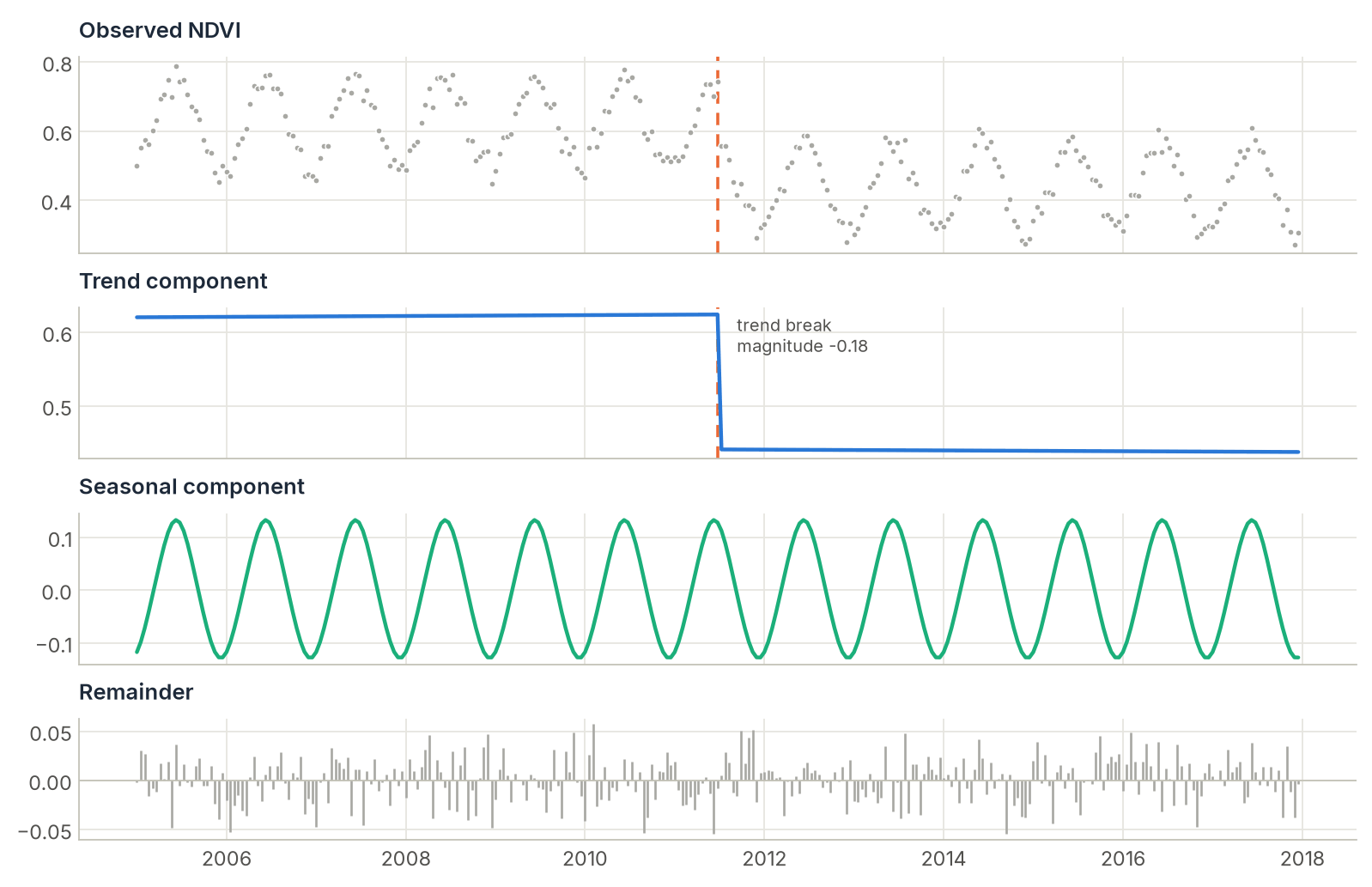
How it works

BFAST decomposes the series as

\[ Y_t = T_t + S_t + e_t \]

(trend, season, remainder) and alternates between two segmented regressions until neither changes:

1. Trend step. Remove the current seasonal estimate and fit a piecewise-linear trend, choosing the number and position of breaks (Bai & Perron, with BIC).
2. Season step. Remove the trend and fit a piecewise harmonic model, again choosing its breaks.

The first seasonal estimate comes from an STL decomposition, as in R. Before each break search, a stability test (OLS-MOSUM) checks whether there is any evidence of change at all. If there isn't, no break is reported.

Compared with BFAST Lite, classic BFAST is slower (several iterations per pixel) but separates trend breaks from seasonal breaks.

Step by step

import zeit

# ndvi_16d: (time, y, x) DataArray of 16-day composites starting in January 2010
ndvi_16d = ndvi_16d.chunk({"time": -1, "y": 256, "x": 256})

result = zeit.bfast(
    ndvi_16d,               # start_time 2010.0 and frequency 23, from the dates
    h=0.15,                 # minimum segment size, fraction of the observations
    max_breaks_trend=5,     # break slots reported for the trend
    max_breaks_season=5,    # break slots reported for the season
).compute()

n_trend = result.n_trend_breaks
n_season = result.n_season_breaks
jump = result.magnitude                  # largest trend jump, 0 if none
when = result.break_time                 # fractional year of that jump

The same function takes a GeoTIFF larger than memory (zeit.bfast("ndvi_16d.tif", chunks="auto")), a numpy array or a single pixel (all inputs), and runs from the shell as zeit bfast. zeit.save_raster(result, "results/bfast") writes one georeferenced GeoTIFF per metric.

Reading the output

The xarray.Dataset has one (y, x) map per metric:

Variable	Meaning
n_trend_breaks	Number of trend breaks at convergence.
n_season_breaks	Number of seasonal breaks at convergence.
magnitude	Size of the largest jump in the trend (difference between the fitted levels either side). 0 if there is no trend break. Matches R's bf$Magnitude.
break_time	Fractional year of that jump, NaN if none. Matches R's bf$jump$x.
n_iter	Iterations until convergence (or max_iter).
n_valid	Valid observations used.
valid	1.0 if the series was long enough to fit (more than 2 × frequency observations).
trend_breakpoint_idx_1 … _k	0-based index (in the whole series, gaps included) of the last observation before each trend break, NaN past n_trend_breaks.
season_breakpoint_idx_1 … _k	Same for seasonal breaks.
trend_magnitude_1 … _k	The jump of the trend at each trend break; magnitude is the largest.
trend_break_date_1 … _k	Date of the first observation after each trend break.

Seasonal amplitude changes are hard to detect

The stability test sums residuals, so a change that only makes the seasonal cycle larger or smaller averages out and is rarely significant. This is a property of the method (R behaves the same way), not a bug. If amplitude changes matter to you, look at CCDC or phenology metrics.

Parameters

Parameter	Default	Effect
start_time, frequency	from the dates	Regular time axis: first observation and observations per year.
order	3	Number of harmonics in the seasonal model.
h	0.15	Minimum segment size, as a fraction of the observations.
max_iter	10	Maximum trend/season iterations.
level	0.05	Significance level of the stability pre-test. Set 1.0 to always search for breaks.
max_breaks_trend, max_breaks_season	5	Break slots in the output.

Implementation notes, validation and performance

Scope. The iterative trend/season loop with BIC-selected breaks (the default of breakpoints() when breaks = NULL), the STL "periodic" seasonal seed, and the OLS-MOSUM stability pre-test. Differences from R: only season = "harmonic" (R's default is "dummy"), only decomp = "stl", and internal NaN gaps are linearly interpolated only to build the STL seed. The segmented fits skip NaNs as usual.

Validation. Compared with R 4.4.2, bfast 1.7.2 and strucchangeRcpp 1.5.4 on four scenarios (trend break, seasonal-amplitude break, no break, both). Break positions, magnitudes (to 4 decimals) and iteration counts matched. With the pre-test disabled (level=1.0) both implementations find the seasonal break at the same observation; with the default level both suppress it.

Performance. A single call takes about 25 ms for 300 observations with 2 iterations, versus about 106 ms in R (about 4×). With n_jobs=-1 on a 20-thread machine, 2,000 pixels take about 4 s instead of 25 s single-threaded.

References

• Verbesselt, J., Hyndman, R., Newnham, G., & Culvenor, D. (2010). Detecting trend and seasonal changes in satellite image time series. Remote Sensing of Environment, 114(1), 106–115. doi:10.1016/j.rse.2009.08.014
• Cleveland, R. B., Cleveland, W. S., McRae, J. E., & Terpenning, I. (1990). STL: A seasonal-trend decomposition procedure based on loess. Journal of Official Statistics, 6(1), 3–73.
• Bai, J., & Perron, P. (2003). Computation and analysis of multiple structural change models. Journal of Applied Econometrics, 18(1), 1–22. doi:10.1002/jae.659
• Chu, C.-S. J., Hornik, K., & Kuan, C.-M. (1995). MOSUM tests for parameter constancy. Biometrika, 82(3), 603–617.
• Zeileis, A., Leisch, F., Hornik, K., & Kleiber, C. (2002). strucchange: An R package for testing for structural change in linear regression models. Journal of Statistical Software, 7(2), 1–38. doi:10.18637/jss.v007.i02
• R packages bfast and strucchangeRcpp.