Segmentation (SNIC)

Group neighbouring pixels with similar histories into compact regions called superpixels, then work with regions instead of pixels. Classifying one mean time series per field removes salt-and-pepper noise and cuts the number of samples by orders of magnitude.

AnswersWhich pixels belong together as one object (field, patch, stand)?

InputAn image or a whole cube: (y, x), (feature, y, x) or (time, band, y, x)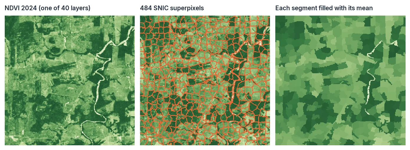

OutputA label map, each segment's mean trajectory, centroids and sizes

ReferenceAchanta & Süsstrunk (2017); the workflow of R sits

Result on real data. A 320 × 320 pixel area of Rondônia segmented on its full 40-year NDVI history (40 features per pixel). Left: one of the 40 layers. Middle: segment boundaries. Right: each segment filled with its mean. Segments follow field edges and the river because they group pixels with similar trajectories, not just similar values on one date. Data: annual Landsat NDVI composites exported from LT-GEE on Google Earth Engine.

Why segment a time series?

zeit.snic works on a single image and on a whole time-series cube: every (time, band) pair becomes one feature, so two pixels are close when their trajectories are close. Two fields with the same average NDVI but opposite seasons fall into different segments. This is the object-based workflow of sits_segment(seg_fn = sits_snic()) in R's sits.

Given the same seeds, Zeit produces the same labels as the authors' reference implementation (github.com/achanta/SNIC), pixel for pixel.

How SNIC works

1. Seeds are placed on a grid. Each seed starts a cluster.
2. A single priority queue holds candidate (pixel, cluster, distance) entries; it starts with every seed at distance 0.
3. The closest entry is popped. If its pixel is still free, it joins that cluster, the cluster's running means are updated, and the pixel's free 4-neighbours are pushed with their distance to the updated cluster.
4. Repeat until every pixel is labelled — one pass, no iterations (unlike SLIC's k-means).

The distance combines feature and image space:

\[ d = \lVert \mathbf{c}_i - \mathbf{c}_k \rVert^2 + \left(\frac{M}{S}\right)^2 \lVert \mathbf{p}_i - \mathbf{p}_k \rVert^2, \qquad S = \sqrt{N / K} \]

where \(\mathbf{c}\) are the features (all bands at all dates), \(\mathbf{p}\) the row/column position, \(N\) the number of valid pixels, \(K\) the number of seeds and \(M\) the compactness.

Choosing compactness

The feature term is in data units, so \(M\) must follow the scale of your data. Small \(M\) follows the data closely (irregular segments); large \(M\) approaches a regular grid. 0.5 is the sits default for reflectance-scaled cubes; the reference implementation's 10 suits 0-255 CIELAB images. If bands have very different ranges, standardise them first — every feature counts equally in the distance.

Step by step

1. Segment a cube

import zeit

cube = zeit.load_raster("ndvi_evi_2022.tif")      # (time, band, y, x), e.g. 23 dates x (NDVI, EVI)
seg = zeit.snic(cube, spacing=10, compactness=0.5, grid="hexagonal")

seg.labels       # (y, x) segment ids, -1 = unlabelled (missing pixels), georeferenced
seg.means        # (segment, time, band): the mean trajectory of every segment
seg.n_pixels     # (segment,) pixel counts
seg.centroid_x   # (segment,) centre of mass, in map coordinates (also centroid_y)

Seeds come from one of two places:

Argument	Seeds
spacing= (+ grid, padding)	the grids of the R snic package used by sits_snic() (snic_grid): "rectangular" (default), "diamond", "hexagonal", "random"; default spacing=10, padding=spacing/2
seeds=	your own (n, 2) (row, col) pixel positions (takes precedence)

The same works on a single map (y, x), a stack (band, y, x) or a raster path, and as cube.zeit.snic(...).

2. Export polygons

gdf = zeit.snic_to_polygons(seg, include_means=True)
# columns: supercells, x, y (centroid), n_pixels, one column per feature (2022-01-01_ndvi, ...), geometry
zeit.save_raster(seg, "results/snic")              # labels.tif

The segment means can go straight to any classifier (TempCNN, LTAE, TWDTW, random forest…) as one sample per segment.

Large images: tiles and parallelism

SNIC is inherently sequential — each step depends on the previous pop — so a single image is segmented on one core. The C++ core is still 1.5–4× faster than the reference C code on one thread (more so with more features) (pixel-major feature layout for contiguous, vectorised Eigen distance computations; float32 input used without a float64 copy), and OpenMP parallelises the data reordering.

For large scenes, use tile_size: the image is split into tiles that are segmented independently and in parallel (OpenMP), each seed belonging to the tile that contains it — the same block-wise strategy sits_segment() uses. Segments never cross tile edges, and labels remain the global seed index, so the output is identical for any n_jobs.

seg = zeit.snic(cube, spacing=10, compactness=0.5, tile_size=512, n_jobs=-1)

Memory: the core keeps one pixel-major copy of each tile being processed (rows × cols × features values of the input dtype) plus the priority queue.

Fidelity to the reference implementation

From the same seeds, the labels match those of snic.c (Achanta, EPFL). That includes how ties are broken: when two clusters reach a pixel at exactly the same cost, the heap's order decides the winner the same way. The test suite gives Zeit the seeds the original placed and compares labels on RGB-like, noisy, piecewise-constant (many ties) and time-series inputs, in float32 and float64. The original's code is not included in Zeit.

Differences from the original:

• Seed grid: seeds come from the sits grids (spacing) or your own list, not from the original's FindSeeds. To compare with the original, pass its seeds explicitly, as the test suite does.
• NaN handling (as in the R snic package used by sits): pixels with a NaN in any feature are left unlabelled (-1), and \(N\) counts valid pixels only. A seed on a NaN pixel gives an empty segment. Gap-fill the cube first (regularize_time_series, apply_whittaker_filter) if you want every pixel labelled.
• Heap bug fix: the reference pop() never removes the heap's last node. With a single seed it reads an uninitialised pixel index and crashes; on tiny images it can return a label that does not exist. Here the heap drains normally.
• No RGB→CIELAB conversion: the reference's optional doRGBtoLAB is specific to 8-bit RGB photos; convert beforehand if you need it.

---

References

• Achanta, R., & Süsstrunk, S. (2017). Superpixels and Polygons Using Simple Non-Iterative Clustering. CVPR 2017, 4651–4660.
• Simoes, R., et al. snic: Superpixel Segmentation with the Simple Non-Iterative Clustering Algorithm (R package), used by sits_snic().
• Simoes, R., Camara, G., et al. (2021). Satellite Image Time Series Analysis for Big Earth Observation Data. Remote Sensing, 13(13), 2428.