Clustering (SOM)

Find the main types of behaviour in a landscape without any labels. A self-organizing map groups millions of pixel trajectories into a small grid of prototypes, each one a typical time series, arranged so that similar prototypes sit next to each other.

AnswersWhich typical trajectories exist here, and where?

InputA cube, a stack or a Dataset of maps: every value of a pixel is a feature

OutputA cluster map, the prototype trajectory of each cluster and each pixel's distance to it

ReferenceKohonen (1990, 2013); bit-exact port of minisom

Result on real data. 40-year NDVI trajectories of 490,000 pixels in Rondônia, clustered by a 2 × 2 batch SOM trained on a sample of 30,000. The prototypes separate a gradient from intact forest (cluster 1) to the land cleared earliest (cluster 4). No labels were used. Data: annual Landsat NDVI composites exported from LT-GEE on Google Earth Engine.

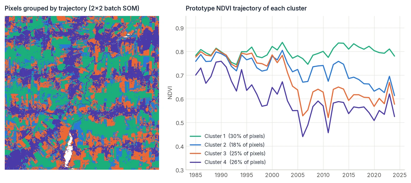
How it works

A SOM is a grid of neurons, each holding a prototype vector with as many values as your features. Training repeatedly finds, for each sample, its closest neuron (its best-matching unit, BMU) and moves that neuron and its grid neighbours toward the sample. The neighbourhood and the learning rate shrink as training goes on. The result is a set of prototypes that covers the data and is topologically ordered: neighbours on the grid are similar.

Zeit implements both forms of the algorithm in C++:

• Online SOM (Kohonen, 1990): one sample at a time, sequential by definition.
• Batch SOM (Kohonen, 2013): every prototype is updated from all samples at once in each pass, parallelised with OpenMP. It is much faster on large satellite data sets.

Its engine, zeit.ai.SOM, is an operation-by-operation port of Python minisom. Given the same seed and arguments it draws the same initial weights and sample order and applies the same arithmetic, so the trained codebook is bit-for-bit identical to MiniSom, 30–190 times faster. See Algorithm Fidelity.

Step by step

1. Cluster a cube

zeit.som takes the cube as it is. Every value a pixel holds off y/x is a feature: each date of an index, each band of each date, or each map of a Dataset (phenology metrics, LandTrendr's event maps...).

import zeit

ndvi = zeit.load_raster("LT_Stack_NDVI_Rondonia.tif")      # (time, y, x), 40 years
clusters = zeit.som(ndvi, x=2, y=2, sample=30_000)

The SOM is trained on a random sample of pixels (sample, reproducible by seed), which is usually enough. Then every pixel goes to its best-matching neuron, block by block if the cube is lazy. Pixels with a missing value (NaN, or the raster's NoData) get no neuron.

sigma is the initial neighbourhood radius in grid units. Small grids (2 × 2, 3 × 3) work as a clustering method. Larger grids (10 × 10 and up) are used to explore the data, or as a first step before grouping neurons.

2. Read the result

clusters.label                       # (y, x): the neuron of each pixel, 1 to x * y (0: no data)
clusters.distance                    # (y, x): distance to the neuron's prototype
clusters.prototypes                  # (neuron, time): one typical trajectory per neuron
clusters.n_pixels                    # (neuron): pixels in each cluster
clusters.attrs["quantization_error"] # mean distance of the sample to its prototypes

clusters.prototypes.sel(neuron=1).plot()
zeit.save_raster(clusters, "results/som")      # label.tif and distance.tif

The prototypes keep the cube's dims and coordinates, so a (time, band, y, x) cube gives prototypes (neuron, time, band). The grid position of each neuron is in the i and j coordinates (minisom's winner). A large distance marks the pixels the map represents poorly, which are often the interesting ones.

3. Look at it

clusters.label.zeit.plot()           # the cluster map, one colour per neuron
zeit.plot(ndvi, fit=clusters)        # click a pixel: its series, with its neuron's prototype

4. Clean labelled samples (optional)

SOMs are also used to check the training data of a supervised classifier: a sample whose class disagrees with the majority class of its neuron is suspicious. zeit.clean_samples trains a SOM on the samples' features and marks each one:

checked = zeit.clean_samples(stack, "samples.gpkg", label="class")
checked[["class", "neuron", "neuron_class", "purity", "keep"]]
rf = zeit.train_classifier(stack, checked[checked.keep], label="class")

purity is the share of the neuron's samples in its majority class: a neuron where two classes mix is a sign that the features cannot tell them apart. This is the idea behind sits_som_clean_samples() in R sits.

Online or batch?

algorithm	Same as minisom	Meaning of num_iters	Parallel
"online" (default)	MiniSom.train(data, num_iters)	Number of single-sample updates (default: 20 passes over the sample)	No (sequential by definition)
"batch"	MiniSom.train_batch_offline(data, num_iters)	Number of full passes over the data (default 20)	Yes (n_jobs)

zeit.som trains online by default. On small grids the batch update can leave neurons empty: a neuron that wins no sample is pulled onto its neighbour's mean and stays there, so two neurons end up identical. The online update does not do this, and on a sample of 50,000 it takes about as long. Batch pays off on large grids and samples, where it runs in parallel.

The engine

zeit.som runs on zeit.ai.SOM, the engine, which you can also use directly on samples you arrange yourself, (samples, features):

from zeit.ai import SOM

som = SOM(x=2, y=2, input_len=X.shape[1], sigma=0.8, learning_rate=0.5, random_seed=0)
som.random_weights_init(X)               # or som.pca_weights_init(X)
som.train(X, num_iters=20, algorithm="batch")
prototypes = som.get_weights().reshape(-1, X.shape[1])
bmu = som.predict(X)                     # flat neuron index i * y + j, from 0 to x*y - 1
keep = som.filter_noisy_samples(X, labels)

train continues from the current weights, like minisom, and batch results are identical for any n_jobs. With sample=None and the same arguments (note that zeit.som lets the learning rate fall to 0, decay_function="linear_decay_to_zero", where the engine and minisom default to "asymptotic_decay"), zeit.som gives exactly the engine's prototypes, and label is som.predict + 1. All the methods are listed in the API reference.

Parameters

Parameter	Default	Effect
x, y	3, 3	Grid size. x * y is the number of prototypes.
sample	50000	Pixels to train on (None: all).
algorithm	"online"	"online" or "batch".
num_iters	None	Updates (online) or passes (batch); default 20 passes.
sigma	1.0	Initial spread of the neighbourhood function.
learning_rate	0.5	Initial learning rate.
decay	"linear_decay_to_zero"	Online: the learning rate falls to 0, so the prototypes settle (minisom's "asymptotic_decay" ends at a third of it).
neighborhood	"gaussian"	"gaussian", "mexican_hat", "bubble" or "triangle".
topology	"rectangular"	"rectangular" or "hexagonal" grid.
init	"random"	"random" (sample pixels), "pca" (first two principal components) or None.
seed	42	Seed of the sample, the initialisation and the sample order.

Good practice

• Scale features consistently. The distance treats every feature equally. If you mix bands with different ranges, standardise them first.
• Fill gaps, or accept that gappy pixels get no neuron. Pixels with a missing value are left out. zeit.smooth fills them.
• Interpret prototypes, not colours. Plot clusters.prototypes to understand what each cluster means, as in the figure above.
• Reproducibility. Results depend on seed, the sample and the initialisation. Fix them, and you get the same result every run, and the same codebook as minisom with the same settings.

References

• Kohonen, T. (1990). The self-organizing map. Proceedings of the IEEE, 78(9), 1464–1480. doi:10.1109/5.58325
• Kohonen, T. (2013). Essentials of the self-organizing map. Neural Networks, 37, 52–65. doi:10.1016/j.neunet.2012.09.018
• Vettigli, G. (2018). MiniSom: minimalistic and NumPy-based implementation of the Self Organizing Map. github.com/JustGlowing/minisom
• R package sits: sits_som_map() and sits_som_clean_samples().