Trend Analysis (Mann-Kendall)
Is this area getting greener or browner, and is the trend real or just noise? The Mann-Kendall test answers the first half without assuming anything about the data's distribution, and the Theil-Sen slope says how fast it is changing. Both are robust to outliers such as residual clouds.
(time, rows, cols)pymannkendall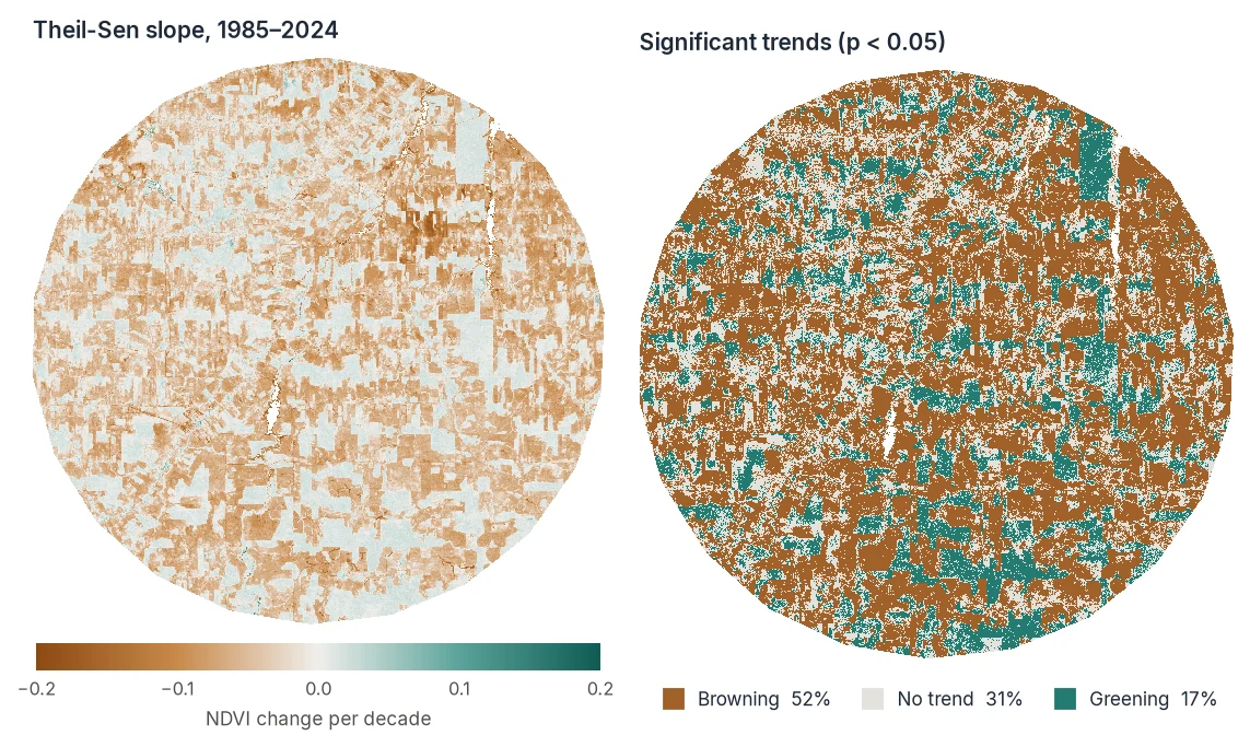
How it works
- Mann-Kendall compares every pair of observations and counts how often the later one is higher. If "later is higher" happens much more often than chance allows, there is an upward trend (and vice versa). It uses only ranks, so it does not care about skewed distributions or a few extreme values.
- Theil-Sen estimates the slope as the median of the slopes between all pairs of points, so outliers barely move it.
Why not a linear regression? Ordinary least squares assumes normal, independent residuals. Satellite series violate both: indices are skewed, consecutive years are correlated, and missed clouds produce outliers.
Step by step
1. Build one value per year
The slope is expressed per time step. With one observation per year, it is directly "change per year":
import zeit

# ndvi: (time, y, x) DataArray from build_time_series, any cadence
annual_max = ndvi.groupby("time.year").max().rename({"year": "time"})   # (years, y, x)
annual_max = annual_max.chunk({"time": -1, "y": 512, "x": 512})
A yearly maximum or growing-season median are common choices.
2. Run the test
result = zeit.mann_kendall(annual_max, method="hamed_rao", alpha=0.05).compute()

slope = result.slope                             # NDVI change per year
significant = result.h == 1                      # significant at alpha
browning = significant & (result.trend == -1)
greening = significant & (result.trend == 1)
The result is an xarray.Dataset with one (y, x) map per metric, on the grid and CRS of the cube. A dask cube gives a lazy result; an in-memory cube an in-memory one.
3. Save the maps
zeit.save_raster(result, "results/mk")                       # slope.tif, p.tif, ... one per metric
zeit.save_raster(browning, "results/browning.tif")           # georeferenced from the cube
Which variant should I use?
method |
Use it when |
|---|---|
"hamed_rao" |
Default and recommended for annual composites. Corrects the test for autocorrelation (a wet year tends to follow a wet year), which otherwise produces too many false trends. |
"yue_wang" |
An alternative autocorrelation correction. Worth comparing when results are borderline. |
"original" |
The classic test, for series you know are independent. |
"seasonal" |
Raw sub-annual data (16-day, monthly). Tests each season slot separately and combines them (Hirsch & Slack), so you don't need to aggregate to one value per year. Set period to the number of steps per year. |
# 16-day composites tested directly: 23 observations per year
trend = zeit.mann_kendall(ndvi_16d, method="seasonal", period=23)
Units of the slope
For original, hamed_rao and yue_wang, the slope is per array step. With 16-day data that is per 16 days, not per year. For seasonal, it is per full period (per year when period covers a year).
Reading the output
| Variable | Meaning |
|---|---|
trend |
1 increasing, -1 decreasing, 0 no significant trend. |
h |
1.0 if significant at alpha, else 0.0. |
p |
Two-sided p-value. |
z |
Standardised test statistic. |
tau |
Kendall's tau, from −1 to 1. |
s, var_s |
Mann-Kendall score and its (corrected) variance. |
slope |
Theil-Sen slope, see the units warning above. |
intercept |
Intercept of the robust line. |
Pixels with fewer than min_valid (default 4) non-NaN values are all NaN.
More ways to call it
zeit.mann_kendall reads what it is given (all inputs):
# A GeoTIFF with one band per year, larger than memory: read and computed block by block
mk = zeit.mann_kendall("LT_Stack_NDVI_Rondonia.tif", chunks="auto")
zeit.save_raster(mk, "results/mk")

# A numpy (time, y, x) array: no dates needed
mk = zeit.mann_kendall(stack)

# One series, for testing: a Dataset of scalars
px = zeit.mann_kendall([0.41, 0.44, 0.39, 0.47, 0.52, 0.49, 0.55, 0.58, 0.61, 0.60])
float(px.slope), float(px.p)
From the shell: zeit mann-kendall.
Good practice
- Trend is not timing. Mann-Kendall says a monotonic trend exists over the whole period, not when it started. Pair it with LandTrendr or CCDC to find when and how abruptly.
- Many pixels, many tests. At
alpha=0.05, about 5% of trendless pixels will still test significant. Look at spatial patterns, or tightenalpha, before interpreting isolated pixels. - Mask what cannot trend. Water and bare ground produce meaningless tests. Mask them first.
Validation
The implementation is a C++ port of pymannkendall and matches it field for field on hundreds of synthetic series, for every variant. See Algorithm Fidelity.
References
- Hussain, M. M., & Mahmud, I. (2019). pyMannKendall: a python package for non parametric Mann Kendall family of trend tests. Journal of Open Source Software, 4(39), 1556. doi:10.21105/joss.01556
- Mann, H. B. (1945). Nonparametric tests against trend. Econometrica, 13(3), 245–259. doi:10.2307/1907187
- Kendall, M. G. (1975). Rank Correlation Methods (4th ed.). Griffin.
- Sen, P. K. (1968). Estimates of the regression coefficient based on Kendall's tau. Journal of the American Statistical Association, 63(324), 1379–1389. doi:10.1080/01621459.1968.10480934
- Hamed, K. H., & Rao, A. R. (1998). A modified Mann-Kendall trend test for autocorrelated data. Journal of Hydrology, 204(1–4), 182–196. doi:10.1016/S0022-1694(97)00125-X
- Yue, S., & Wang, C. (2004). The Mann-Kendall test modified by effective sample size to detect trend in serially correlated hydrological series. Water Resources Management, 18(3), 201–218. doi:10.1023/B:WARM.0000043140.61082.60
- Hirsch, R. M., & Slack, J. R. (1984). A nonparametric trend test for seasonal data with serial dependence. Water Resources Research, 20(6), 727–732. doi:10.1029/WR020i006p00727