BFAST Lite

Find how many structural changes happened in a whole time series, and when. BFAST Lite splits each pixel's history into the statistically optimal number of segments, each with its own trend and seasonal cycle, in a single fast pass.

AnswersHow many breaks does this series have, and where are they?

InputA regular series of one index; gaps as NaN

OutputNumber of breaks and the index of each break per pixel

ReferenceMasiliūnas et al., R package bfast (bfastlite)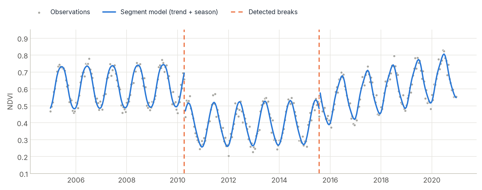

What BFAST Lite produces. A synthetic 16-day NDVI series with a drop in 2010 and a partial recovery from 2015. BFAST Lite finds both breaks. The blue lines are a trend-plus-season model refitted within each segment, for display.

How it works

BFAST Lite fits the model response ~ trend + harmonics to the series and searches for the set of breakpoints that minimises the total error, using the Bai & Perron dynamic program. Adding breaks always lowers the error, so the number of breaks is chosen with an information criterion (LWZ by default) that penalises extra segments. Each segment must hold at least a fraction h of the observations.

Unlike the classic BFAST, it needs no seasonal decomposition and no iteration, and it handles missing values natively. Unlike BFAST Monitor, it looks at the whole series retrospectively.

Step by step

import zeit

# ndvi_16d: (time, y, x) DataArray of 16-day composites starting in January 2010
ndvi_16d = ndvi_16d.chunk({"time": -1, "y": 256, "x": 256})

result = zeit.bfast_lite(
    ndvi_16d,               # start_time 2010.0 and frequency 23 (16-day steps), from the dates
    h=0.15,                 # each segment holds >= 15% of the observations
    max_breaks=5,           # report at most 5 breaks per pixel
).compute()

n_breaks = result.n_breaks
first_break = result.breakpoint_idx_1                  # NaN where n_breaks == 0

To turn a break index into a date, for a series without gaps:

first_break_time = result.attrs["start_time"] + first_break / result.attrs["frequency"]   # fractional year

The same function takes a GeoTIFF larger than memory (zeit.bfast_lite("ndvi_16d.tif", chunks="auto")), a numpy array or a single pixel (all inputs), and runs from the shell as zeit bfast-lite. zeit.save_raster(result, "results/bfl") writes one georeferenced GeoTIFF per metric.

Reading the output

The number of breaks varies by pixel, so the output reserves max_breaks slots and fills the unused ones with NaN. The xarray.Dataset has one (y, x) map per metric:

Variable	Meaning
n_breaks	Number of breaks chosen by the criterion (0 if none).
rss	Residual sum of squares of the selected model.
lwz	Value of the LWZ criterion that was minimised.
n_valid	Valid (non-NaN) observations used.
valid	1.0 if the series had enough observations to fit.
breakpoint_idx_1 … _k	0-based index of the last observation before each break, in chronological order, NaN past n_breaks.
magnitude_1 … _k	The model after each break minus the model before it, both on the first observation after the break.
break_date_1 … _k	Date of the first observation after each break, NaT past n_breaks.

Indices count every observation

Break indices refer to the whole series, missing observations included, so cube.time[idx] is the date of the last observation before the break even when the pixel has gaps. break_date_k already gives the first date after it, and extract_events turns the breaks into a map of one event per pixel, as for LandTrendr and CCDC.

Parameters

Parameter	Default	Effect
start_time	from the dates	Time of the first observation, as a fractional year.
frequency	from the dates	Observations per year.
order	3	Number of seasonal harmonics.
h	0.15	Minimum segment size as a fraction of the valid observations. Larger values forbid short segments.
max_breaks	5	Number of break slots in the output.

Implementation notes, validation and performance

Scope. The default breaks="LWZ" model selection over response ~ trend + harmon, with the segment RSS table computed from recursive residuals (O(n²) rather than O(n³)).

Validation. Compared with R's bfastlite() on six scenarios (a single break, no break, two candidate breaks, NaN gaps, monthly data, non-default h). All six matched n_breaks and every break position exactly; rss differed by 1e-6 to 1e-7.

Performance. On 300 pixels of 150 observations, R bfastlite() took 34.5 ms per pixel and Zeit 11.2 ms single-threaded (about 3×). With n_jobs=-1 on 15 of 16 cores, 20,000 pixels took 45.5 s instead of 249.3 s single-threaded (a further 5.5×). The gain is smaller than BFAST Monitor's because the dynamic program is real computation on both sides, not interpreter overhead.

References

• Masiliūnas, D., Tsendbazar, N.-E., Herold, M., & Verbesselt, J. (2021). BFAST Lite: A lightweight break detection method for time series analysis. Remote Sensing, 13(16), 3308. doi:10.3390/rs13163308
• Bai, J., & Perron, P. (2003). Computation and analysis of multiple structural change models. Journal of Applied Econometrics, 18(1), 1–22. doi:10.1002/jae.659
• Liu, J., Wu, S., & Zidek, J. V. (1997). On segmented multivariate regression. Statistica Sinica, 7(2), 497–525.
• Brown, R. L., Durbin, J., & Evans, J. M. (1975). Techniques for testing the constancy of regression relationships over time. Journal of the Royal Statistical Society, Series B, 37(2), 149–163.
• R packages bfast and strucchangeRcpp.