Monitoring with EWMACD

EWMACD watches every observation of a pixel with a control chart, the tool factories use to notice when a machine drifts. A harmonic model learns the pixel's normal seasonal cycle from a few stable years. After them, the chart follows how far each new observation falls from the model, and it signals when the departures add up. Because it works date by date, it takes irregular, cloudy Landsat series as they are, without compositing, and it catches subtle, lasting changes such as thinning as well as clear-cuts.

AnswersSince when has this pixel left its normal behaviour, how far, and has it come back?

InputEvery observation of one index, irregular dates welcome: (time, y, x)

OutputThe flags of every date; maps of the first disturbance, its severity, the recovery, the first gain and the state at the last date

ReferenceBrooks et al. (2014), IEEE Transactions on Geoscience and Remote Sensing 52(6)

What EWMACD produces. Two real pixels of the sample data of Brooks et al. (2014): the tasseled cap angle index of loblolly pine stands in Alabama, 51 Landsat dates from 2005 to 2011. Top: the observations and the harmonic model fitted on the training years (shaded); hollow dots are training dates screened out as clouds or shadows. Bottom: the EWMA of the residuals and its control limits. Orange dots are dates flagged as disturbed. Left: a drop from early 2009, deepest in August 2010, back within the limits in December 2010. Right: a sharp drop in February 2010, most likely a harvest, still far below the model in October 2011.

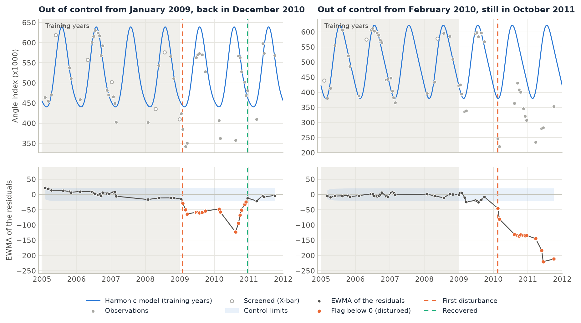
How it works

1. Learn the normal cycle. For each pixel, a constant plus order (2) sine and cosine pairs of the day of the year is fitted to the observations of the training years. Dates more than xbar_train (1.5) standard deviations from this first fit are dropped as clouds and shadows (a Shewhart X-bar chart), and the model is fitted again without them.
2. Compute the residuals. Every date gets its residual: observation minus model. After the training years, only gross anomalies, beyond xbar_monitor (20) standard deviations, are dropped, so that real changes stay in.
3. Smooth them in a control chart. The exponentially weighted moving average (EWMA) of the residuals, z = (1 - lmbda) * z_previous + lmbda * residual, remembers the recent dates, so that a small shift that lasts adds up while a single odd date fades. Its control limits are sigmas (3) standard deviations of the EWMA, from the training residuals.
4. Flag. Each date's flag is the EWMA divided by its limit, truncated: 0 inside the limits, -1, -2... for a loss of one, two... limits, and positive values for a gain. A signal must last persistence (3) dates to count.

From the flags after the training years come the maps: the first disturbance, its severity, the date it came back, the first gain, and the state at the last date.

Step by step

The data are the sample data of the paper, a 65 x 64 pixel stack of the tasseled cap angle index (x 1000) over loblolly pine stands in Alabama, USA (Virginia Tech data repository). Its 51 dates are uneven: 11 in 2006, 4 in 2007 and 4 in 2011.

1. Load every date

import zeit

cube = zeit.load_raster("ewmacd_sample/angle_*.tif")   # one GeoTIFF per date, the date in the name
cube.sizes                                              # time: 51, y: 64, x: 65

The download is a single stack with its dates in a CSV file. Give them to load_raster:

import pandas as pd

t = pd.read_csv("Temporal Distribution with DOY.csv")
dates = pd.to_datetime(dict(year=t.Year, month=t.Month, day=t.Day))
cube = zeit.load_raster("Sample Data - Angle Index x1000 Stack.tif", dates=dates)

Use every observation, with the clouds masked as NaN, and do not composite: EWMACD needs the dates as they are. Any vegetation index works (NDVI, NBR, EVI); the paper uses the tasseled cap angle, atan(greenness / brightness).

2. Run EWMACD

The paper trains on 2005-2008 and monitors 2009-2011. train_end is the first year after the training period:

res = zeit.ewmacd(cube, train_end=2009)

list(res.data_vars)
# ['flags', 'break_time', 'severity', 'recovery_time', 'gain_time', 'state', 'sigma', 'rmse', 'r2', 'coefficients']

The 4,160 pixels take 40 ms. The training years must be stable: a pixel disturbed during them has a poor model and signals at once when monitoring starts.

3. Read the maps

Result of this tutorial. Left: the angle index on the last date; the pale patch, cleared in 2010, is most likely a harvest. Middle: the date of the first disturbance, for the pixels whose disturbance reached 3 control limits or more. Right: the state at the last date.

Variable	Meaning
flags	(time, y, x): the chart's flag at every date. 0 in control, negative a loss, positive a gain, in control limits.
break_time	The first disturbance after the training years, as a decimal year (NaN: none).
severity	Its most negative flag until it came back: -3 is three control limits below the model.
recovery_time	The first date back inside the limits (or above) after the disturbance.
gain_time	The first positive flag after the training years.
state	At the last date: 0 stable, 1 disturbed, 2 recovered (disturbed, then back), 3 gain.
sigma, rmse, r2	The training residuals' standard deviation behind the limits, and the model's fit.
coefficients	(coefficient, y, x): the harmonic model's constant, sines and cosines.

names = res.state.attrs["flag_meanings"].split()   # ['stable', 'disturbed', 'recovered', 'gain']
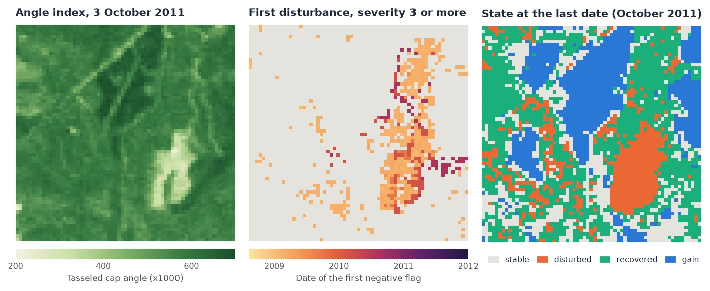
res.state.to_series().value_counts()               # 0: 888, 1: 636, 2: 1648, 3: 988

severe = res.break_time.where(res.severity <= -3)  # the map in the middle
zeit.save_raster(res[["break_time", "severity", "state"]], "results/ewmacd")

The maps show how sensitive the method is. 2,284 pixels (55%) have a first disturbance, and 82% of them start in the first months of 2009: half of the scene drifts below its model in the spring of 2009, by one or two limits, and most of it comes back (57% of these pixels within 2009, 86% by 2011). That is why so many pixels are "recovered" at the last date. It is a weak, widespread signal, more likely weather than management. The severe changes are fewer: 15% of the pixels have a first disturbance of severity 3 or more, grouped in stands, and 5% are at -3 or less on the last date, most of them in the harvest (85% of them have an angle index below 450 in October 2011, against a median of 574 over the scene). Filter on severity, as in the middle map, to keep the clear changes.

The pixels in gain (24%) have an index that stays above their training model, as a young stand that keeps growing would.

4. Look at one pixel's chart

With one pixel's series, the result also has the chart itself, date by date: ewma, limit and fitted (the model).

px = zeit.ewmacd(cube.isel(y=39, x=50), train_end=2009)   # the harvested pixel, right in the first figure
float(px.break_time), int(px.severity), int(px.state)     # (2010.13, -10, 1)

(px.ewma / px.limit).plot.line("o")                       # out of control beyond -1 and 1

ewma and limit are NaN on the dates that were screened out of the chart. Those dates carry the flag of the date before.

Other inputs

The same function takes a raster on disk, a numpy array or a single pixel (all inputs):

# many GeoTIFFs, read and computed block by block
res = zeit.ewmacd("landsat_ndvi/*.tif", train_end=2017, chunks="auto")
zeit.save_raster(res[["break_time", "severity", "state"]], "results/ewmacd")

# one pixel's series: a pandas Series indexed by date, or values with dates=
px = zeit.ewmacd(series, train_end=2017)
px = zeit.ewmacd(values, train_end=2017, dates=dates)

Parameters

Parameter	Default	Effect
train_end	required	The first year after the training period. The model is fitted on the years before it.
train_start	first year	Dates before it are left out.
order	2	Sine and cosine pairs of the harmonic model.
lmbda	0.3	Weight of each new residual in the EWMA, in (0, 1]. Lower: a slower, smoother chart, more weight on lasting shifts. 1 charts each date on its own.
sigmas	3.0	The control limits, in standard deviations of the EWMA. Higher: fewer and later signals.
persistence	3	Dates a signal must last. Counted in dates, not in time: in a cloudy year, 3 dates can span months.
xbar_train	1.5	Training dates beyond this many standard deviations are screened out of the model.
xbar_monitor	20.0	Later dates beyond this many standard deviations are screened as anomalies. Raise it for smooth series (see below).
low	None	Values not above it are missing: fill values, water, bare soil.

Good practice

• Expect short false signals with the defaults. Screening the training dates at 1.5 standard deviations makes sigma smaller than the noise, so the limits are tight: the chart sees small changes, and it also signals briefly on noise. On a synthetic series of stable forest (Gaussian noise only, 145 dates, example 24), 24% of the pixels got a short signal with the defaults, nearly all of -1; 4% with persistence=6, none with persistence=12; 6% with sigmas=4 or xbar_train=2.5. With each of these settings, a thinning that lowered the index by twice the noise was still found in every pixel, a median of one or two months after it. Brooks' later scripts use half the dates of a year as the persistence.
• Mask clouds before. Missing dates are fine. A dark date that the cloud mask missed is not: after the training years, only residuals beyond xbar_monitor are screened, and a cloud shadow is often less than that. It enters the EWMA and weighs on it for several dates (with lmbda=0.3, 70% of it remains on the next date). Mask with the QA band, or with Tmask.
• Raise xbar_monitor for smooth series. A clear-cut larger than 20 standard deviations of a very quiet pixel is screened as an anomaly until it comes back within them, which delays the detection.
• Check the training years. A pixel disturbed during them signals at once after them, and its r2 is low.
• Read severity, not only break_time. The first disturbance can be a flag of -1. The deeper and longer ones are the changes worth mapping.

About this implementation

The flags are those of Brooks' EWMACD v1.3.0 R script, the paper's own; Earth Engine has the method as ee.Algorithms.TemporalSegmentation.Ewmacd. With persistence=1 they were checked date by date on synthetic series and on 400 pixels of the sample data used here. With more persistence, the first disturbance is the same, and a few later dates differ where the script, which means to keep the previous lasting state, reads another date's flag. Values not above low are missing from the start, whereas the script still fits them in its first regression. On 10,000 pixels and 71 dates, the script takes 2.8 s, and Zeit 55 ms on one thread and 7 ms on 19. See Against the Original Implementations.

For a regular series and a statistical test of the break, see BFAST Monitor. For degradation in the tropics from the fractions of each observation, see CODED.

References

• Brooks, E. B., Wynne, R. H., Thomas, V. A., Blinn, C. E., & Coulston, J. W. (2014). On-the-fly massively multitemporal change detection using statistical quality control charts and Landsat data. IEEE Transactions on Geoscience and Remote Sensing, 52(6), 3316–3332. doi:10.1109/TGRS.2013.2272545
• Sample data and the EWMACD R script: Brooks, E. B., Virginia Tech. doi:10.7294/W4WD3XHK