Benchmarks & accuracy¶

Landschaft makes two promises: the same results as the established tools, and much less waiting for them. This page shows how both are checked, with the numbers.

Same results

The tools are compared with the programs they reproduce: pixel for pixel, value for value, or to a stated tolerance where the original itself works in floating point. The exceptions are listed below.
Faster

C++ with OpenMP (and Eigen for the circuit solver): from a few times to hundreds of times faster than the originals.
Tested on every change

The comparisons live in the test suite: stored outputs of the originals, and live runs when the original is installed.

Speed¶

Speed-up over the original tools

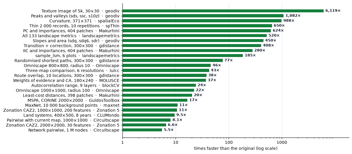
How much faster Landschaft is than the tool it reproduces, on the cases in the tables below (logarithmic scale). The original's time is its own run, including its input and output where noted; Landschaft is timed in memory.

How these were measured

The MSPA table was measured with tools/benchmark.py (version 0.53), and the spatial prioritization table with tools/benchmark_prioritize.py, on a desktop Intel Core i5-13600K (14 cores, 20 threads, 64 GB, Windows 11), the fastest of 10 alternating runs, with both programs kept on the performance cores. The other timings were recorded in the changelog when each tool was written, with the version given ("Since"). Times depend on the computer, the map and the options: treat them as orders of magnitude.

Habitat patterns (MSPA)¶

Against GuidosToolbox's mspa executable (v2.3, whose time includes reading and writing its TIFF files) on its sample map and on the CORINE forest map; Landschaft with 1 thread and with the default 19. Every output was compared pixel by pixel. Landschaft is 10 to 17 times faster.

Map	Connectivity, edge width	GuidosToolbox	1 thread	19 threads	Identical
Sample, 1000²	8, 1	0.46 s	0.040 s	0.029 s	yes
Sample, 1000²	8, 5	0.56 s	0.065 s	0.054 s	yes
Sample, 1000²	4, 20	0.68 s	0.079 s	0.068 s	yes
CORINE, 2000²	8, 1	1.30 s	0.095 s	0.078 s	yes
CORINE, 2000²	8, 5	1.53 s	0.151 s	0.137 s	yes
CORINE, 2000²	4, 20	1.70 s	0.213 s	0.174 s	yes

At scale, the CORINE map repeated 3 × 3 (6000 × 6000, 36 million pixels) takes GuidosToolbox 20 to 26 s and Landschaft 1.4 to 2.3 s, again with identical outputs.

MSPA's longest steps (geodesic distances, thinning, watershed) are ordered propagations that must run in sequence to stay bit-exact, so one map takes only 10 to 30 % less time with more threads. Many maps gain fully: run them side by side with mspa_batch or batch.

Hybrid processors

On processors with performance and efficiency cores (Intel 12th generation and later), Windows may move a busy process to the slower efficiency cores, especially when it runs in the background; any program then takes up to twice as long. Keep the terminal in the foreground for timings, and compare runs made side by side.

Landscape metrics¶

Against the R package landscapemetrics 2.2.2.

Task	landscapemetrics (R)	Landschaft	Since
All 133 metrics of `augusta_nlcd` (440 × 678)	15.6 s	0.03 s	0.14
`sample_lsm`, 6 plots of `augusta_nlcd`	3.7 s	0.02 s	0.15
Nearest-neighbour distances (`enn`) of `augusta_nlcd`	2.4 s	0.014 s	0.14
`get_nearestneighbour`, 1000 × 1000	1.8 s	0.05 s	0.18

At scale: a 10,000 × 10,000 map with 7.7 million patches gets all 133 metrics (92 million values) in about 10 s, and maps larger than memory are read in blocks with the same results.

Habitat networks¶

Against the R package Makurhini (and, through it, gdistance).

Task	Makurhini (R)	Landschaft	Since
IIC and node importances, 404 patches (`MK_dPCIIC`)	1.4 s	0.005 s	0.30
PC and node importances, 404 patches (`MK_dPCIIC`)	10.6 s	0.017 s	0.30
Least-cost distances, 398 patches over 222 k cells	10.2 s	0.5 s	0.32
Commute-time distances		13 × faster	0.39

At scale: the 35 million centroid distances between 8,395 patches of a 4000 × 4000 map take 0.9 s, and all 4.3 million links of a 5,000-patch PC graph are rated in 22 s.

Circuit connectivity¶

Against Omniscape 0.7 and Circuitscape 6.1 (Julia), both with 20 threads.

Task	Original	Landschaft	Since
Omniscape, 800 × 800, radius 10	29.4 s	0.64 s	0.43
Omniscape, 700 × 700, radius 25	46.7 s	1.36 s	0.43
Omniscape, 1000 × 1000, radius 100	275 s	12.4 s	0.43
Circuitscape pairwise, 1000 × 1000, 20 focal points	8.7 s	2.7 s	0.48
… with the cumulative current map	76.5 s	9.5 s	0.48
Circuitscape one-to-all with maps, same map	21.8 s	4.6 s	0.48
Circuitscape network pairwise, 1 M nodes, 20 focal nodes	27.7 s (CHOLMOD), 182 s (default cg+amg)	5.0 s	0.51

Every window and every circuit is solved exactly (a sparse Cholesky factorisation), and the result does not depend on the number of threads.

Grid distances¶

Against the R package gdistance 1.6.5 on a 300 × 300 grid of random resistances (8 directions; best of 3 runs in R, of 5 in Landschaft).

Task	gdistance (R)	Landschaft	Since
Transition (`1 / mean`) and geographic correction	2.0 s	0.005 s	0.75
Cost surface from one point (`accCost`)	0.10 s	0.011 s	0.76
Least-cost distances between 20 points	0.31 s	0.026 s	0.76
Least-cost paths to 5 goals	0.05 s	0.012 s	0.76
Commute distances between 10 points	0.29 s	0.084 s	0.77
Random-walk passages	0.36 s	0.066 s	0.77
Randomised-shortest-path passages (`theta = 0.5`)	5.98 s	0.078 s	0.80
Randomised-shortest-path distances, 3 × 3 points	fails (a 60 GiB dense matrix)	0.15 s	0.80
… the same on 60 × 60	0.23 s	0.0043 s	0.80
Route overlap from a common origin, 10 locations	5.97 s	0.16 s	0.79

At scale: on 2000 × 2000 (4 million cells) a transition takes 0.15 s, a cost surface 0.6 s, a random-walk passage map 4.5 s, a randomised-shortest-path passage map 4.6 s (7.8 s for an asymmetric transition).

Neutral landscape models¶

The same landscapes as NLMR (same seeds, identical values), one model call each (best of 5, default threads).

Task	NLMR (R)	Landschaft	Since
`nlm_random`, 2000 × 2000	0.25 s	0.044 s	0.54
`nlm_percolation`, 1000 × 1000	1.54 s	0.014 s	0.54
`nlm_planargradient`, 2000 × 2000	0.25 s	0.017 s	0.54
`nlm_edgegradient`, 2000 × 2000	0.31 s	0.020 s	0.54
`nlm_distancegradient`, 2000 × 2000	0.25 s	0.10 s	0.54
`nlm_distancegradient`, 360 × 90 (great-circle distances)	0.06 s	0.011 s	0.54
`landscape_classify` by proportions, 1000 × 1000	0.05 s	0.019 s	0.54
`nlm_mpd`, 1025 × 1025	0.13 s	0.043 s	0.55
`nlm_neigh`, 500 × 500	0.04 s	0.023 s	0.55
`nlm_randomrectangularcluster`, 300 × 300, sides 5–20	0.02 s	0.003 s	0.55
`nlm_randomcluster`, 200 × 200	19 s	0.003 s	0.56
`nlm_curds`, 512 × 512 (three steps)	0.03 s	0.003 s	0.56
Gaussian field (`simulate_gaussian_field`), 500 × 500	0.36 s	0.043 s	0.57
Fractional Brownian motion (`simulate_fbm`), 1000 × 1000	0.40 s	0.050 s	0.57
`nlm_mosaicfield`, 200 × 200, 20 mosaics	9.95 s	0.010 s	0.58
`nlm_mosaicfield`, 100 × 100, 20 mosaics and the limiting field	9.0 s	0.008 s	0.58
`nlm_mosaictess`, 500 × 500, 1000 germs	0.25 s	0.010 s	0.59
`nlm_mosaicgibbs`, 500 × 500, 500 germs	0.50 s	0.007 s	0.59

Surface metrics¶

Against geodiv 1.1.1 and spatialEco 2.0-5 (R 4.4.2, terra 1.9-50) on geodiv's example rasters (371 × 371 cells: normforest, orforest for the trend, orelevation for terrain), measured with tools/benchmark_surface.py: the best of 3 runs in R (fast tasks repeated to 0.5 s), of 5 in Landschaft with the default threads. Where Landschaft corrects geodiv or spatialEco the work is the same.

Task	R	Landschaft	Since
Amplitude (sa, sq, ssk, sku)	29 ms	3.9 ms	0.85
Best trend surface of order 0-3	0.15 s	25 ms	0.85
Slopes and developed area (sdq, sdq6, sdr)	2.16 s	4.8 ms	0.85
Peaks and valleys (sds, ssc, s10z)	1.84 s	1.7 ms	0.85
Bearing area parameters (sbi, sci, svi, sk, spk, svk)	0.88 s	11 ms	0.85
Correlation lengths and aspect ratio (scl, stxr)	0.13 s	28 ms	0.85
Texture direction and wavelength (std, srw)	0.61 s	28 ms	0.85
Fractal dimension (sfd)	6.3 ms	2.2 ms	0.85
Texture image, Sa in 5 × 5 windows, 100 × 100 (`focal_metrics`)	0.17 s	1.0 ms	0.85
Texture image, Sk in 5 × 5 windows, 30 × 30 (`focal_metrics`)	134 s	22 ms	0.85
TPI, 5 × 5	8.5 ms	2.5 ms	0.88
TRI	0.97 s	1.9 ms	0.88
VRM	80 ms	15 ms	0.86
Curvature (total)	1.58 s	1.6 ms	0.88
Hierarchical slope position, scales 3-27	0.11 s	14 ms	0.88
Spherical standard deviation	73 ms	12 ms	0.86

The gains are largest where the R packages compute cell by cell in R (texture images, peaks, curvature, TRI) and smallest where terra's focal functions do the work in C++ with running sums (TPI, HSP, VRM). Landschaft's focal means, sums and standard deviations use compensated prefix sums along the rows (within about 1e-13 of summing each window), so a window costs one step per row whatever its size.

Terrain hydrology¶

Against WhiteboxTools 2.4 on a rough terrain of 3000 × 3000 cells, both on 4 cores (tools/benchmark_hydro.py, best of 3); WhiteboxTools' times include reading and writing its GeoTIFFs, so Landschaft's include writing its result.

Task	WhiteboxTools	Landschaft	Since
Filling depressions	3.16 s	2.07 s	1.48
Least-cost breaching (channels up to 20 cells)	3.86 s	2.35 s	1.48
D8 flow accumulation	1.95 s	0.62 s	1.48
D-infinity flow accumulation	1.84 s	1.22 s	1.48
FD8 flow accumulation	2.00 s	1.65 s	1.48

Spatial prioritization¶

Against Zonation 5 v2.4 (z5.exe, and z5_16bit.exe for 16 bits) on synthetic species maps: seeded Gaussian random fields above a threshold, each feature on 60 % of the cells (10 % in the 200-feature case), written as GeoTIFFs. Measured with tools/benchmark_prioritize.py (version 0.95) on the performance cores, one run of z5 and the fastest of 3 of Landschaft; both times include reading the GeoTIFFs, and z5's writing its outputs. Every rank map is the same, bit for bit, as z5's on one thread.

Map	Features	Rule	Iterations	z5, 1 thread	z5, 12 threads	Landschaft, 1 thread	Landschaft, 12 threads	Since
1000 × 1000	30	CAZ2	60	20.6 s	12.4 s	9.5 s	1.86 s	0.95
2000 × 2000	30	CAZ2	60	102.8 s	48.0 s	45.6 s	7.29 s	0.95
2000 × 2000	30	ABF	20	53.6 s	23.4 s	36.5 s	5.90 s	0.95
2000 × 2000	30	CAZ2, 16 bits	60	104.4 s	49.7 s	46.2 s	8.71 s	0.95
1000 × 1000	200 sparse	CAZ2	59	105.8 s	33.6 s	15.0 s	3.16 s	0.95

On one thread Landschaft is 1.5 to 7 times faster than z5, most with many sparse features: each feature is walked along its own occurrences, where z5 visits every feature in every cell. With 12 threads the gap grows to 4 to 11 times: z5 gains 1.7 to 3 times from its 12 threads, Landschaft 4.7 to 6.3. Memory: about 130 bytes per cell with data during the ranking, plus 1 to 2 bytes per value that is not zero; storage= puts the large arrays in memory-mapped files.

Optimized plans¶

Against prioritizr 8.0.6's models solved by HiGHS 1.15 alone (the solver prioritizr calls) and by Gurobi 12, on synthetic problems of tools/benchmark_optimize.py: 30 species-like features with targets of 30 % and costs from 1 to 10 (multi-action: 10 features, 3 threats), a gap of 1 %, 12 threads on the performance cores. "No answer" means no plan within the time limit (120 s unless stated). The same models and the same optima as prioritizr's; Landschaft's engines start HiGHS from near-optimal plans, fix the units whose choice is proven, and solve the problems general solvers find hard on their own.

Problem	Units	HiGHS alone	Gurobi	Landschaft	Since
minimum set	10⁵	7 s	2 s	0.44 s	1.21
minimum set	10⁶	no answer (its best plan 2.1 x the optimum)	20 s	1.7 s (gap 0.002 %)	1.21
minimum set	10⁷ (5 features)			60 s, proven optimal	1.26
boundary penalty	10⁶	no answer in 16 min	289 s	27 s (gap 0.77 %)	1.21
minimum penalties with boundary, gap 10 %	2400	more than 150 s		12 s	1.27
multi-action, least cost	10⁵	57 s	3 s	0.7 s	1.22
multi-action, least cost, gap 0	10⁵	no answer in 300 s	13 s	6 s	1.22
multi-action with boundaries	10⁴		7.5 s	0.18 s	1.22
multi-action with river dependencies (soft / hard)	10⁵		6 s / 8 s	1 s / 5.5 s	1.22

Contiguity constraints are the exception. prioritizr's contiguity model is a restriction (it misses some patches, see the migration guide); Landschaft solves the exact model, starting from a patch of the restricted one and with directed cuts added before the branch and bound. On prioritizr's contiguity test problems (166 units, a raster and a table) it proves a gap of 5 % in 1 to 1.5 s and finds patches as cheap as or cheaper than prioritizr's optimum. On larger problems the bound stays weak without cuts inside the branch and bound: on Serra Verde at 3 km (543 units, 8 features) Landschaft's network after 120 s is 4.6 % above the best Gurobi finds in 600 s, with a proven gap of 17 % (Gurobi's, 3.8 %).

Species distributions¶

Against the R packages each step reproduces (R 4.4.2, terra 1.9-50): CoordinateCleaner 3.0.1, spThin 0.2.0, usdm 2.1-7, dismo 1.3-16, blockCV 3.2-0, predicts 0.1-19, ecospat 4.1.3 and maxnet 0.1.4 with glmnet 4.1-10. The inputs are the example climate (9 bioclimatic layers, 192 × 186 cells of 0.5°), the Bradypus records with 10 000 background points, 5 000 synthetic records over the same area and 2 000 clustered ones. Measured with tools/benchmark_sdm.py (version 1.0) on the performance cores: the best of 3 runs in R (fast tasks repeated to 0.5 s), of 5 in Landschaft with the default threads. Every result is the same as R's, the random steps included (same seed), except where the notes on accuracy below say otherwise.

Task	R	Landschaft	Since
Clean 5 000 records: capitals, centroids, equal, GBIF, institutions, outliers, zeros (CoordinateCleaner)	1.99 s	0.16 s	1.0
Thin 2 000 records at 10 km, 10 repetitions (spThin)	0.91 s	1.4 ms	1.0
VIF selection, 9 layers (usdm `vifstep`)	0.17 s	16 ms	1.0
10 000 background points (dismo `randomPoints`)	0.43 s	12 ms	1.0
Hexagonal blocks of 500 km, 10 116 points, 100 iterations (blockCV `cv_spatial`)	1.77 s	53 ms	1.0
k-means folds, 10 116 points, 25 starts (blockCV `cv_cluster`)	93 ms	14 ms	1.0
Autocorrelation range, 9 layers, 5 000 cells each (blockCV `cv_spatial_autocor`)	17.5 s	0.73 s	1.0
Evaluate 1 000 presences against 10 000 background points (predicts `pa_evaluate`)	0.19 s	8.3 ms	1.0
Boyce index, the same predictions (ecospat)	9.8 ms	1.6 ms	1.0
MESS, 9 layers, 10 116 reference points (predicts)	0.75 s	19 ms	1.0
MaxNet, 116 presences and 10 000 background points, 9 predictors (maxnet)	3.25 s	0.30 s	1.0

The largest gains are where R works on whole matrices: spThin computes the distance between every pair of records and rescans them after each removal (Landschaft keeps only the neighbours, in a grid over the sphere, and the counts in a tree: a million records take seconds, where R runs out of memory), and blockCV's blocks and predicts' evaluation go through data frames row by row. MaxNet keeps glmnet's arithmetic and order of operations, so the gain comes from screening (most gradient checks are settled by a bound, without the exact dot product) and from parallel work around the coordinate descent, which itself stays serial; with 20 predictors and hinge features (10 000 background points) it fits in 0.47 s against R's 6.4 s. Weighted sampling without replacement, which R does in time proportional to the cells times the draws, runs in closed form over runs of equal weights (1 million cells and 30 000 draws: 0.24 s against 16-20 s with R's algorithm).

Land change simulation¶

Against the land change tools ls.simulate reproduces, on the cases of its reference tests. Measured with tools/benchmark_simulate.py (version 1.20): lulcc 1.0.4 in R 4.4.2 (with the corrections of tools/lulcc_fixed.R, so that both sides make the same allocation; only the timed call is measured), MOLUSCE 5.3.0's algorithms in Python, Dinamica EGO 8.13's console (the time of a script that only loads the maps is subtracted); the best of 3 runs, the default threads. CLUMondo and FUTURES were timed when they were written.

Task	Original	Landschaft	Since
CLUE-S allocation, Plum Island, 14 steps (lulcc `allocate`)	36.4 s	4.12 s	1.8
Ordered allocation, Plum Island, 14 steps (lulcc `allocate`)	2.9 s	0.40 s	1.8
Land systems, 400 × 500 cells, 8 years (CLUMondo)	16.2 s	1.7 s	1.9
Urban growth, 600 × 800 cells, 5 steps (`r.futures.simulation`)	0.35 s	0.20 s	1.10
Weights of evidence and 3 simulator iterations, 180 × 240 (MOLUSCE)	1.99 s	53 ms	1.15
Three-map comparison, agreement budget and figure of merit, Plum Island, 6 resolutions (lulcc)	7.21 s	0.17 s	1.17
Fuzzy similarity of the differences, windows 1-11, 480 × 640 (Dinamica EGO)	0.67 s	49 ms	1.18
Gravity potential, 1000 × 1000, 1000 sources (Dinamica EGO `CalcInteractionPotentialMap`)	0.42 s	0.13 s	1.46
Stock taken by patches, 3000 × 3000, 50 000 cells (Dinamica EGO `PatcherContinuousState`)	3.8 s	0.59 s	1.46
Cost surface to a road network, 3000 × 3000 (Dinamica EGO `CalcCostMap`, passes until exact)	769 s	1.4 s	1.46

The Dinamica EGO functors of version 1.46 were timed with tools/benchmark_dinamica.py on 4 cores on both sides (Dinamica with -processors 4), the time of the functor in Dinamica's log. Its cost surface sweeps the map in four directions until no cost changes (fewer passes give an approximation); Landschaft's runs Dijkstra's algorithm once, with the same sums.

CLUE-S draws a random number per cell and class at each of its thousands of passes, from R's generator, one after the other: Landschaft draws the same numbers, so the gain is in the rest of the pass. The three-map comparison runs lulcc's equations per block in one pass of C++ (R builds a raster per class and equation), and MOLUSCE loops over the pixels in Python.

Zonal statistics and extraction¶

Not a reproduction of another tool: the functions that read a raster in zones and at points (zonal_stats, extract), against the Python packages commonly used for it, rasterstats 0.21 and exactextract 0.3 (both single-threaded). A 5000 × 5000 float32 raster in memory; the statistics mean, min, max, standard deviation and median; random polygons of 16 vertices. Measured with tools/benchmark_zonal.py (version 0.98) on the performance cores, the fastest of 3 alternating runs.

Case	rasterstats	exactextract	Landschaft, 1 thread	Landschaft, 12 threads	Since
zonal statistics, 2000 small polygons (16 million cells)	2.34 s	3.59 s	0.37 s	0.16 s	0.98
zonal statistics, 20 large polygons (22 million cells)	1.14 s	8.37 s	0.37 s	0.18 s	0.98
values at 1 million points	~119 s	–	0.028 s	0.014 s	0.98

The cells of every polygon are those GDAL burns (the centre rule, or all_touched), as rasterstats takes them: the statistics agree with its own, which adds up in single precision, to 1e-7, and with NumPy in double precision to 1e-15. exactextract weights every cell by the share of it the polygon covers, so its means differ slightly. The median and the percentiles take a linear-time selection, not a sort; the result does not depend on the number of threads.

Plotting¶

ls.plot, from the data to the page a notebook or a window shows (the map's HTML, images and data included), measured with tools/benchmark_plot.py (version 1.32.0) on the performance cores, the fastest of 3 runs. A first plot in a session also imports folium and compiles its templates, about 0.7 s once. A page holds everything it needs (Leaflet, about 0.16 MB; plotly, 4.3 MB, in a page with charts), so it opens without a network connection.

Case	Time	Page
float32 raster, 10 000 × 10 000, in memory	0.25 s	4.7 MB
class raster, 10 000 × 10 000, in memory	0.14 s	1.6 MB
float32 raster, 10 000 × 10 000, read lazily from a file	0.61 s	4.7 MB
float32 raster, 2000 × 2000	0.23 s	5.1 MB
stack of 47 bands of 1000 × 1000 (a band per thread, 16 million pixels in all)	0.85 s	14 MB
10 000 polygons coloured by a column (GeoJSON)	0.14 s	2.7 MB
50 000 polygons coloured by a column (WebGL)	0.36 s	1.5 MB
200 000 polygons coloured by a column (WebGL, with their columns)	0.99 s	5.3 MB
2 million points coloured by a column (WebGL)	0.70 s	13 MB
50 000 polygons, static figure (`static=True`, drawn as a PNG)	0.57 s	0.7 MB
200 000 polygons, static figure (burnt into an image)	0.80 s	0.6 MB
a table of landscape metrics (a chart)	0.03 s	4.3 MB

The time hardly grows with the size of a raster: it is reduced to the resolution of the screen first (block means in C++, or the cells of a lazy raster read in strips), and only that is reprojected and encoded.

Accuracy¶

How results are compared¶

Stored references. The outputs of the original tools on the example maps, on synthetic maps built to hit edge cases, and on the originals' own test cases are stored in tests/data/reference. Every run of the test suite compares with them.
Live runs. When the original is installed, the tests also run it on freshly generated random maps and compare on the spot (pytest -m live_reference).
Original code, not a re-reading of it. Where GuidosToolbox computes in IDL, its processing statements are copied verbatim from guidostoolbox.pro and run with GDL, the free IDL implementation, with GuidosToolbox's own spatcon, grayspatcon, recode and ggeo programs where it calls them.
Bits, then tolerances. Integer maps and counts must be identical. Floating-point results are compared bit for bit where the original's arithmetic can be reproduced (landscapemetrics: R's 80-bit sums and x87 log/sqrt), and otherwise to the tolerance given below, typically the precision of the original itself.

Results by tool¶

Tools	Compared with	Agreement
MSPA	GuidosToolbox `mspa` v2.3 executable: sample map with 7 parameter sets, 10 synthetic scenes, live random scenes; during development 1,200 random cases and CORINE with edge widths up to 100	identical, 0 differing pixels
MSPA Tiling	GuidosToolbox's IDL code with its GDAL tools and `mspa`, in GDL	identical
SPA, Accounting	GuidosToolbox's IDL code in GDL	identical maps and statistics
FAD, FAD-MS, FOS, landscape mosaic, contagion and clustering	GuidosToolbox's IDL code and `spatcon` / `grayspatcon` / `recode`	identical maps; single-precision means and standard deviations to 1e-4 (Landschaft computes in double)
FAD-MS change, landscape mosaic heatmap and heatmap change	GuidosToolbox's IDL code in GDL	identical
Isochrone maps A and AB, least-cost path	GuidosToolbox's `ggeo` and IDL post-processing	identical
133 landscape metrics and the utilities	landscapemetrics 2.2.2 (R): 14 maps (its example data, NA cells, non-square cells, degenerate layouts) × 5 option sets, live random maps	identical bits; `gyrate` and rare `enn` ties to a relative 1e-10; `circle` is randomised in landscapemetrics
FRAGSTATS extras, `convention="fragstats"`, spatial signatures	pylandstats, scikit-learn, FRAGSTATS' definitions	same values
Habitat graphs: indices, node and link importances, centrality	Makurhini (`MK_dPCIIC`, `MK_dPCIIC_links`, `MK_RMCentrality`) and Conefor Sensinode 2.2 / 2.7.1	Makurhini: unrounded values to 1e-12, its rounded output exactly; Conefor: to its single precision (6 digits)
Nodes and distances (centroid, edge, least-cost, commute-time)	Makurhini's `nodesfile` / `distancefile` (gdistance)	identical bits; commute-time to 1e-11
ProtConn, grids, ECA change, focal nodes	Makurhini (`MK_ProtConn`, `MK_Connect_grid`, `MK_dECA`, `MK_dECA_grid`, `MK_Focal_nodes`)	its rounded tables exactly; ECA change to 1e-13
Settlement probabilities (SAMC)	samc and Makurhini's `MK_dPC_SAMC`	1e-14
Omniscape	Omniscape 0.7 with the CHOLMOD solver: its test configurations and synthetic maps	1.7e-11
Circuitscape raster modes	Circuitscape 6.1 with CHOLMOD: its own test cases (advanced, 17 pairwise, 25 one-to-all / all-to-one)	advanced: currents to 1.2e-13 of the largest; pairwise: resistances to 1e-12, maps to 3e-13; one-to-all: 5e-14
Circuitscape network mode	Circuitscape's network test cases and six synthetic ones	1.1e-14
Grid distances: transitions (4/8/16 directions, symmetric or not, R's arithmetic, Mahalanobis), geographic correction (projected, longitude/latitude, global grids), normalisation, arithmetic, cost surfaces, least-cost distances and paths	gdistance 1.6.5 (R 4.4.2, raster 3.6-31, igraph 2.1.3): 53 reference cases, among them uniform grids where many paths cost the same	identical bits and the same paths
Grid distances: commute distances, random-walk and randomised-shortest-path passages and distances, route overlap, barrier and area transitions	the same gdistance: 15 reference cases	1e-14 typical, 1e-10 worst (different sparse factorisations than R's Matrix package); barrier and area transitions identical
Surface metrics: amplitude parameters (`sa`, `sq`, `ssk`, `sku`, `sv`, `sph`, `smean`), trend surfaces of order 0-3 and the choice of the best one, slopes and developed area (`sdq`, `sdq6`, `sdr`), peaks, valleys, `sds`, `ssc`, `s10z`, the bearing area curve and its parameters (`sdc`, `sbi`, `svi`, `sci`, `sk`, `spk`, `svk`), autocorrelation, correlation lengths, texture direction and wavelength, fractal dimension, texture images	geodiv 1.1.1 (R 4.4.2, terra 1.9.50, spatial 7.3-17), and where geodiv errs geodiv with its errors corrected (`tools/surface_fixed.R`): 70 reference cases, projected and longitude/latitude, among them geodiv's example rasters, NA cells, non-square cells and ties	identical bits
Terrain indices: slope, aspect, tpi, tri, vrm, srr, dissection, curvature, spherical standard deviation, hsp, trasp, hli	spatialEco 2.0-5 and terra 1.9-50 (R 4.4.2), and where spatialEco errs spatialEco with its errors corrected (`tools/surface_fixed.R`): 3 DEMs (square and rectangular cells, missing cells, longitude/latitude)	identical bits; focal means (tpi, hsp, srr, vrm, spherical standard deviation, Bolstad's curvature) within 1e-12 of summing each window (compensated prefix sums), 1e-11 of terra's running sums; on longitude/latitude slope and aspect within 1e-12
Terrain hydrology: least-cost breaching, D8 and D-infinity directions, D8, D-infinity and FD8 accumulations (cells, specific contributing area), HAND, wetness, stream power and sediment transport indices	WhiteboxTools 2.4: 4 DEMs (SRTM, missing cells, rectangular cells, terraced elevations with many flats and ties)	identical bits (the accumulations and indices to the float32 WhiteboxTools writes); filling and breaching identical to `FillDepressions` and `BreachDepressionsLeastCost` (on one thread) run with the map's edge as an outlet (WhiteboxTools raises depressions that touch the edge or missing cells, and leaves channels to the edge uncut)
Terrain hydrology: multiple flow routing (`"mfd"`), distance to channel, stream tracing, its D8 routing, pit filling	pygeoprocessing 2.4.11 (the routing of InVEST 3.20): the same 4 DEMs, plain and weighted	identical bits
Spatial prioritization: the ranking (8 rules, weights and weight groups, output groups, thresholds, zero modes, value extraction, costs, hierarchic masks, analysis areas, smoothing, 8 and 16 bits), condition, retention, pre-processing maps, transformed layers, connectivity transforms, post-processing, impact assessment	Zonation 5 v2.4 (`z5.exe`, `z5_16bit.exe`, on one thread): 64 reference projects, and the timing cases below	identical rank maps and iterations; curve, statistics, post-processing and impact files digit for digit
Optimized prioritization: every objective, target, penalty, constraint, decision and portfolio of prioritizr; raster, table and polygon planning units	prioritizr 8.0.6 (R 4.4.2; its errors corrected: phylogenetic tip order, portfolio cuts): `compile()` of 55 reference problems; the optimum with Gurobi	identical models, row by row and bit for bit; the same optima
Evaluation: summaries, representation, target coverage, Ferrier, rarity-weighted richness, replacement and rank importance; calibration	prioritizr 8.0.6 and its calibration vignette	identical bits (R's `pnorm` ported)
Multi-action planning	prioriactions 0.5.0 (its errors corrected): `getModelInfo` of 6 reference problems, costs, benefits, actions	identical models and figures; the same optima as Gurobi; dependencies and portfolios tested against exhaustive enumeration
Polygon planning units	exactextractr 0.10.0 (`exact_extract(fun = "sum")`)	identical cell fractions and sums
Marxan	Marxan 4.0.6 (its errors corrected), the same seeds	identical runs: solutions, scores, summaries
Species distributions: occurrence cleaning (all 13 tests, records on circle vertices, the antimeridian and poles), thinning, one record per cell	CoordinateCleaner 3.0.1 (its errors corrected: `tools/cc_fixed.R`), spThin 0.2.0, terra 1.9-50: 14 reference cases	identical flags and kept records; the circles' vertices identical (GeographicLib 2.7 and 1.52 with mingw's x87 maths)
Species distributions: predictor selection, background points, spatial blocks and clusters, ENMeval partitions	usdm 2.1-7, dismo 1.3-16, blockCV 3.2-0 (its own k-means: R's `kmeans`, 48 cases), ENMeval 2.0.5.2: 53 reference cases with R's generator	identical bits, random steps included
Species distributions: evaluation, Boyce index, omission rates, MESS, MOP	predicts 0.1-19, ecospat 4.1.3 (its errors corrected: `tools/ecospat_fixed.R`), ENMeval, mop 0.1.4: 16 reference cases	identical bits; the p-value of the correlation to 1e-9 (R's `pt`)
Species distributions: Mahalanobis distances (MOP, ExDet), autocorrelation range	mop, dsmextra 1.1.6 (its covariate index corrected), blockCV `cv_spatial_autocor` (automap, gstat 2.1-6)	1e-9 (R inverts the covariance with LAPACK); variograms identical, fitted ranges to 1e-6
MaxNet	maxnet 0.1.4 with glmnet 4.1-10: 13 fits (Bradypus and synthetic, every feature class, regularisation multipliers, factors)	identical bits: coefficients, lambda, entropy and the four output types, on Windows and Linux
Neutral landscape models: random, percolation, gradients, midpoint displacement, fractional Brownian motion, Gaussian fields, Poisson line and Voronoi mosaics, random, neighbourhood and rectangular clusters, curds, classification	NLMR 1.4.0 (R 4.4.2) with the same seeds; R's generator and the libstdc++ distributions of NLMR's C++ code against R and the Rtools compiler	identical bits
Land change analysis: cross tables, intensity analysis, components of difference, multiple resolutions, Markov chains	lulcc 1.0.4, OpenLand 1.0.5, diffeR 0.0-8 (R 4.4.2; their errors corrected, `tools/differ_fixed.R`): 11 cases; Dinamica EGO 8 transition matrices: 6 cases	identical bits; Dinamica's matrices to 2e-11 (it writes 15 digits; its root of the matrix is less exact)
Land change: weights of evidence (ranges, weights, correlations, probabilities)	Dinamica EGO 8.13 (its code is closed: inferred from its outputs): 9 cases, 84 range probes	ranges and counts identical, weights to the 15 digits it writes
Land change: logistic regression, CLUE-S and ordered allocation, neighbourhoods, rules	R's `glm` and lulcc 1.0.4 (its errors corrected: `tools/lulcc_fixed.R`): 9 cases	identical bits, R's random numbers included
Land change: land systems (CLUMondo)	CLUMondo (GitHub a5c0c1f, built Win32 with MSVC; its age error corrected: `tools/clumondo_fixed.patch`): 6 cases; the May 2017 executable for its later options	identical maps and iteration logs; 97-100 % of the cells for the 2017 options (no source)
Land change: urban growth (FUTURES): simulation, flooding, demand, pressure, patch library and calibration	`r.futures` addons in GRASS 8.3.2 (their errors corrected: `tools/futures_fixed.patch`): 16 cases; the potential's mixed model against lme4 2.0.1 and MuMIn 1.48	identical maps and tables; mixed-model coefficients to 2.6e-6 (an optimiser: lme4 stops at its tolerance)
Land change: MOLUSCE's weights of evidence, simulator, multi-criteria evaluation, kappa and error budget	MOLUSCE 5.3.0 imported without QGIS (its confidence corrected: `tools/molusce_fixed.patch`): 6 cases	identical bits, NumPy's random numbers included
Land change validation: three maps at several resolutions, agreement budget, figure of merit, `r.futures.validation`	lulcc 1.0.4 (raster 3.6-31): 2 cases; GRASS's addon: 3 cases	identical bits
Land change validation: fuzzy similarity and similarity of differences	Dinamica EGO 8.13 (measured): 36 maps, windows 1-11, exponential and constant decay	identical maps; means to the 15 digits it writes
Land change: gravity potential (`surface.gravity`)	Dinamica EGO 8.13 `CalcInteractionPotentialMap` (measured): 10 maps, five exponents, with and without a mask	within 3e-6 (Dinamica adds float32 terms in float32; Landschaft sums in float64)
Land change: roads (`friction_cost`, `pathways`)	Dinamica EGO 8.13 `CalcCostMap` and `CalcPathwayMap` (measured): real and integer frictions, with and without diagonal costs, relative frictions, impassable and unreachable cells; paths down the costs and along the directions	identical costs and paths; directions identical except between equally cheap predecessors (Dinamica's follow its sweeps)
Watershed model (`hydro.swat.run`): weather and generator, HRUs (snow, ET, curve number runoff, MUSLE, percolation, lateral flow, nutrients, plant growth, scheduled management, decision tables, crop rotations, urban land), routing units, aquifers, SWAT-DEG channels, every printed table	SWAT+ 62.0.1 built with flang 22 against the UCRT (equal to the official Windows executable in every printed digit), dumping its state each day and its printed records: the official Hubbard Brook and Ames examples, Muskingum routing, two projects made by `from_rasters` (one with crop rotations and urban land) and the plants' minimum C (`c_factor="plant"`)	identical bits (every field of every day)
Watershed division and project files (`hydro.swat.watershed`, `from_tables`)	QSWAT+ 3 (its sources) and the SWAT+ Editor 4.0.2 run on the same tables: a synthetic watershed and a 282 km² DEM (QSWAT+'s test data)	the Editor's 64 files, token for token

The default solver of Omniscape and Circuitscape (conjugate gradients with an algebraic multigrid) is itself only about 2e-7 away from the exact solution; Landschaft's solves are exact, so it is compared with their exact (CHOLMOD) runs.

Checked in other ways¶

These tools follow GuidosToolbox's method, but are not compared with a run of its code:

Tools	How they are checked
Network components and importance of MSPA cores and bridges	an independent step-by-step reproduction of GuidosToolbox's IDL routine
Spatial entropy	an independent reproduction of GuidosToolbox's `entropy_mspainp.pro`
Restoration status, parcellation	GuidosToolbox's values for its sample map
Cost distance, least-cost path, restoration corridor, contortion, simple and morphological change, FOS change, GraySpatCon metrics other than those of FOS	unit tests on constructed cases
Zonal statistics, extraction at points, clip, rasterize	cells against GDAL's rasterizer, statistics against NumPy and rasterstats
Land change: Dinamica's Expander and Patcher	Dinamica EGO 8.13's functors crash for patches of more than one cell, so their seed selection was measured with one-cell patches (acceptance by neighbours, draw by probability) and the patch growth follows the publications; statistical comparison
Land change: Dinamica's continuous Patcher (`ContinuousPatcher`) and road destinations (`destinations`)	Dinamica EGO 8.13's continuous Patcher crashes for patches of more than one cell, as its Patcher does: the candidates, the pruning, the quota and the draw by probability were measured with one-cell patches (exact on the cases that do not depend on the draw, statistical on 32 draws), the growth is the Patcher's; destinations compared statistically on 100 draws (Dinamica's draw errors corrected, see below)
Hilltop protection areas (`surface.hilltop`)	written from the Forest Code (Lei 12.651/2012): Dinamica EGO's `CalcHilltop` follows the older CONAMA 303/2002 rule on a DEM cut into elevation bands, with its own definitions (its slope criterion measures to the map's edge or to other features: 5° on an isolated cone of 21.8°), so only the heights are compared (to 0.05 m on cones); checked against an independent computation of the landforms by connected components on random DEMs, and on cones, ranges and lakes of known geometry
Land change: PLUS's CA with multi-type random patch seeds (CARS)	PLUS is distributed without source code or licence: written from its paper, checked by its properties (demand met, growth from patches and seeds, the threshold, the rules, the same maps with any number of threads)
Land change: dynamic variables, regional demands, presets, projections, scenarios, calibration	unit tests: the pieces they assemble are compared above

Known differences

Euclidean distance, distance to resistance, influence zones and proximity depend on IDL's MORPH_DISTANCE, which does not always pick the nearest object near the boundaries between the zones of different objects (about 1 % of the pixels of the test cases). Landschaft's distances are exact Euclidean distances, so these maps can differ from GuidosToolbox's in detail; influence zones and proximity are marked experimental.
MSPA Tiling reproduces GuidosToolbox's tiling exactly, including its approximation near the tile seams when objects are larger than the overlap. A map that fits in one tile gets the MSPA of the whole map (GuidosToolbox drops the first overlap / 2 columns).
Zonation 5's curves (performance curves, AUC, features_info, histograms and flexibility maps) come from the order of its second-to-last sort, while its rank map comes from the last one. Landschaft's describe the rank map it returns; they are compared with z5 evaluating that rank map (LOAD mode). Flexibility maps are identical where the two orders give the same curves, and otherwise compared with a direct reproduction of Zonation's algorithm.
Zonation 5 on several threads adds up the layers per thread, and its results can differ from its run on one thread; Landschaft's do not depend on the threads and equal z5's on one thread.
Species distributions keep the R packages' results except where they err (each case listed in IDEAS.md and in the functions' notes). Three of the corrections change values people compare with R: the continuous Boyce index drops ecospat's "+1" on the last window (which made the index depend on the scale of the predictions), country checks use Natural Earth's iso_a3_eh (with iso_a3, France and Norway are "-99"), and MOP's Mahalanobis distance uses the reference's covariance (mop used that of the cells tested).
Dinamica EGO's destinations (destinations, of its road constructor): Dinamica gives each quadrant n // q rows or columns, so the last n % q never get a destination, and rounds its draw to an integer of the summed attraction, so the first cell of a quadrant gets half its share and a draw past the end takes the quadrant's last cell, even of no attraction. Landschaft's quadrants cover the map and its draw follows the attraction exactly.
Off Windows, the arctangent of the slopes of surface.terrain is the C library's, as terra's is on Windows: R takes it from Windows' UCRT, whose code is not public, and other C libraries (glibc) differ from it in the last bit. The slopes then differ from R's by one unit in the last place (two in degrees). The SWAT+ port calls the C library's exp, log and powers as SWAT+ does, and carries their last bits through years of daily state: off Windows its results are within 1e-4 of each quantity's scale of SWAT+'s on Windows (2.4e-5 at most in the test cases). Everything else gives the same bits on Windows and Linux: Landschaft carries its own versions of the functions whose bits matter (log, sqrt, sin, cos, atan2, exp and powers as mingw-w64 computes them on the x87 unit, and the UCRT's hypot).

Reproduce¶

The comparisons are part of the test suite:

pip install -e ".[test]"
pytest                              # every test, stored references included
pytest -m live_reference            # also run the originals that are installed

The live runs look for the originals in these environment variables:

Variable	Original
`LANDSCHAFT_MSPA_EXE`	GuidosToolbox's `mspa` executable (`MSPAstandalone/mspa_win64.exe`)
`LANDSCHAFT_GDL_EXE`	GDL, to run GuidosToolbox's IDL code
`LANDSCHAFT_SPATCON_EXE`, `LANDSCHAFT_GRAYSPATCON_EXE`, `LANDSCHAFT_GGEO_EXE`	GuidosToolbox's helper programs
`LANDSCHAFT_RSCRIPT`, `LANDSCHAFT_R_LIBS`	R with landscapemetrics and Makurhini
`LANDSCHAFT_JULIA`, `LANDSCHAFT_JULIA_PROJECT`	Julia with Circuitscape and Omniscape

tools/make_reference*.py regenerate the stored references from the originals, and python tools/benchmark.py --exe <mspa executable> repeats the MSPA timings. tools/make_reference_optimize.py and tools/benchmark_optimize.py use R with prioritizr, prioriactions and gurobi (LANDSCHAFT_RSCRIPT, LANDSCHAFT_R_LIBS); Marxan's references come from its executable in WSL. tools/make_reference_prioritize.py and tools/benchmark_prioritize.py look for Zonation 5's z5.exe and z5_16bit.exe in LANDSCHAFT_Z5_DIR. tools/make_reference_sdm.py and tools/benchmark_sdm.py use R with the packages listed above in LANDSCHAFT_SDM_R_LIBS (default %LOCALAPPDATA%/R/landschaft-sdm-lib). tools/make_reference_simulate.py and tools/benchmark_simulate.py use R with lulcc, OpenLand and diffeR (LANDSCHAFT_SIM_R_LIBS, default %LOCALAPPDATA%/R/landschaft-sim-lib), CLUMondo (LANDSCHAFT_CLUMONDO, LANDSCHAFT_CLUMONDO_FIXED), GRASS 8 with the r.futures addons in WSL, Dinamica EGO's console (LANDSCHAFT_DINAMICA) and MOLUSCE's sources (LANDSCHAFT_MOLUSCE, LANDSCHAFT_MOLUSCE_FIXED); tools/benchmark_dinamica.py times the Dinamica EGO functors added in 1.46 on 4 cores.