Chapter 12.6

Trade-offs and alternatives¶

Every plan is a compromise: between cost and compactness, between money and the share of every species protected, between what one group wants and what another needs. A single "optimal" map hides these compromises. This chapter shows how to bring them into the open: trade-off curves, objective ways of choosing a point on them, and sets of alternative plans that are almost equally good.

In this chapter

calibrating a penalty: the blended and hierarchical approaches, the knee and TOPSIS;
Cohon's trade-off rate as a starting value;
the Pareto front between budget and representation;
portfolios of near-optimal plans, and what they say about flexibility;
scenarios, phased plans and sensitivity analysis.

Calibrating a penalty¶

Chapter 12.5 showed that a boundary penalty buys compactness with money, and that its value has units and must be calibrated. Calibrating means solving the problem for a range of values and choosing one on the resulting curve of cost against boundary. ls.prioritize offers the two approaches of prioritizr's calibration guide (Hanson et al. 2025) and two ways to choose.

The blended approach¶

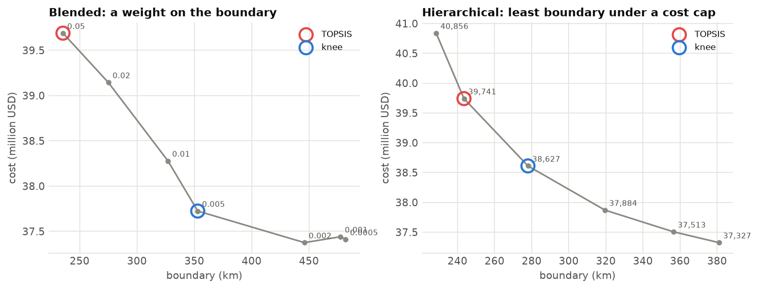
Solve with several penalty values; every value gives a plan with some cost and some boundary:

import numpy as np
import landschaft as ls

P = ls.prioritize
cost = ls.load_raster(P.example_data("cost"))
features = ls.load_raster(P.example_data("features"))
p = P.problem(cost, features).add_min_set_objective().add_relative_targets(0.3).add_binary_decisions()

cal = P.calibrate_penalty(p.add_highs_solver(gap=0.02), "boundary", values=[0.001, 0.003, 0.01, 0.03])
cal.table[["value", "cost", "boundary", "topsis", "knee"]].round(1)

The candidates are solved in parallel. The table marks two choices:

the knee of the curve (Satopää et al. 2011): the point farthest from the straight line between the two ends, where the curve bends most. Before it, compactness is cheap; after it, expensive;
TOPSIS (Hwang & Yoon 1981): the candidate closest to the ideal (least cost and least boundary) and farthest from the anti-ideal, after scaling both criteria. With equal weights it tends to pick a more balanced, often more compact, point than the knee.

best = cal.best("knee")
print(f"knee: penalty {cal.table.loc[cal.table['knee'], 'value'].iloc[0]}, cost {best.cost:,.0f}")

In plain words

The knee answers "up to where is compactness a bargain?". TOPSIS answers "which plan is the best all-rounder, if cost and compactness matter equally?". Neither is the answer; both are defensible, reproducible starting points for a discussion.

The hierarchical approach¶

The blended approach mixes two quantities in one objective, and its penalty values have no direct meaning. The hierarchical approach asks a clearer question in two steps: first, what is the least cost of meeting the targets? Then, how compact can the plan be if we accept spending 1 %, 2 %, 5 % ... more?

hier = P.calibrate_budget(p.add_highs_solver(gap=0.05, time_limit=180), "boundary",
                          inflation=[0.005, 0.01, 0.02, 0.04, 0.07, 0.1])
hier.table[["value", "cost", "boundary", "topsis", "knee"]]

Each candidate is a minimum penalties problem (add_min_penalties_objective): the least boundary that meets every target within a budget. These problems are harder than the blended ones, which is why the example gives a time limit; on large maps, run them on coarser blocks first.

Blended and hierarchical calibration — Calibrating the boundary penalty of Serra Verde's 30 % plan. Left: the blended approach, labelled by the penalty value. Right: the hierarchical approach, labelled by the cost cap (thousand USD). Both curves fall steeply at first: the first million USD above the minimum cost removes far more boundary than the next ones. The circles mark the candidates TOPSIS and the knee choose.

A starting value: Cohon's method¶

Where to start the search? Cohon et al. (1979) proposed the slope between the two extremes: the least-cost plan (ignoring the boundary) and the least-boundary plan (ignoring the cost). The ratio of their differences in cost and boundary is a penalty at which neither criterion dominates. cohon_penalty computes it, and calibrate_penalty without values searches from 1/100 to 100 times it. Finding the least-boundary plan is a hard problem on a fine grid, so the example uses blocks of 6 x 6 km. The value it gives holds for problems on those blocks only: on a coarser grid the cost of a unit grows faster than its boundary (36 times against 6 times here), so the useful penalties are much larger than on the 1 km grid.

c, f = P.coarsen(cost, features, 6)
coarse = P.problem(c, f).add_min_set_objective().add_relative_targets(0.3).add_binary_decisions()
value, ideals = P.cohon_penalty(coarse.add_highs_solver(gap=0.05))
print(f"Cohon penalty on 6 km blocks: {value:.4g}")
ideals.round(0)

Money against representation¶

The minimum set answers one question: what does it cost to meet every target? Decision makers often ask the reverse: what do we get for 10, 20 or 30 million? The Pareto front answers it by solving the minimum shortfall problem (chapter 12.4) for a range of budgets:

front = P.pareto_front(p, n=6)
front.table[["value", "cost", "shortfall", "met"]].round(2)

The Pareto front of budget and shortfall — What each budget buys in Serra Verde. The total shortfall (the sum, over the eight features, of the share of each target still missing) falls quickly at first and slowly at the end: the first millions cover the cheap, common habitat; the last ones buy the dear coastal land of the mangrove and the tamarin. The labels count the targets fully met. That count does not always rise with the budget, because minimum shortfall reduces the total gap, not the number of targets met.

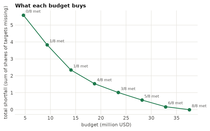
Every point of the front is efficient (Pareto-optimal): no plan is both cheaper and closer to the targets. Points off the front are dominated, and choosing among the points on it is a political decision, not a technical one. The front makes that decision informed.

Alternative plans¶

The optimal plan is rarely the only good one. Often hundreds of plans cost within 1 % of the optimum, and they may differ a lot in where they are. Showing only one hides this flexibility, and stakeholders may reject a plan for a reason that a near-identical alternative would avoid. A portfolio is a set of good plans:

Portfolio	What it returns
`add_gap_portfolio(n, pool_gap)`	up to n distinct plans within `pool_gap` of the optimum (from the solver's pool)
`add_cuts_portfolio(n)`	the best plan, then the best that differs from it, and so on (each forbids the earlier ones)
`add_top_portfolio(n)`	as cuts, each solved to optimality: the n best plans
`add_shuffle_portfolio(n)`	the problem solved with its units in random orders: plans of equal quality when there are ties

port = p.add_gap_portfolio(10, pool_gap=0.02).add_highs_solver(gap=0.01).solve()
print(len(port), "plans; costs from", round(port.summary["cost"].min()), "to", round(port.summary["cost"].max()))
f = port.frequency.values
print("units in every plan:", int(np.nansum(f == 1)), " in some plans:", int(np.nansum((f > 0) & (f < 1))))

The selection frequency (port.frequency) is the share of the plans that select every unit. Units in every plan are hard to replace; units in a few are interchangeable. It is a simple, intuitive measure of irreplaceability, and chapter 12.7 compares it with formal ones.

Scenarios and sensitivity¶

A plan depends on choices that could reasonably be different: targets, costs, weights, data. Good practice is to solve scenarios and keep the priorities that hold across them. Since every add_ method returns a new problem, scenarios are a loop:

scenarios = {
    "30 % of everything": p,
    "60 % of the rare ones": p.add_relative_targets([0.3, 0.3, 0.3, 0.3, 0.6, 0.3, 0.3, 0.6]),
    "area instead of cost": P.problem(cost * 0 + 1, features).add_min_set_objective()
                              .add_relative_targets(0.3).add_binary_decisions(),
}
plans = {k: q.solve() for k, q in scenarios.items()}
for k, s in plans.items():
    print(f"{k:22s} {int(s.values.sum()):4d} cells, {np.nansum(cost.values * s.selection.values):9,.0f}")

For any other parameter, calibrate(make, values, criterion) builds the same kind of trade-off table: make(value) returns the problem for every value (a feature weight, a target, a cost layer), and criterion(problem, solution) measures what is traded against the cost.

Plans in phases¶

Protected areas are created over years, not at once. iterative_solve solves, changes the problem, and solves again, optionally keeping what earlier steps protected. For instance, 20 % by 2026, 25 % by 2028 and 30 % by 2030, each step building on the last:

def next_step(step, solution, problem):
    return problem.add_relative_targets(0.2 + 0.05 * (step + 1))

phases, table = P.iterative_solve(p.add_relative_targets(0.2), next_step, 3, lock_previous=True)
table[["step", "cost", "units"]].round(0)

Phased plans cost a little more than a plan made at once for the final target, since early choices can't be undone. The steps can also take their input from a land-use simulation: chapter 14's ls.simulate changes the landscape between phases, and protected_cells passes the protected cells to it as areas where land use may not change.

Key points

Penalties are calibrated by solving over a range of values and choosing on the curve: the knee or TOPSIS give reproducible choices.
The hierarchical approach asks a clearer question: how compact can the plan be for x % more cost?
The Pareto front shows what every budget buys; choosing a point on it is a political decision.
Many plans are almost as good as the optimum. Portfolios show them, and their selection frequency shows which places are hard to replace.
Solve scenarios, and trust the priorities that hold across them.

Check your understanding¶

The knee of a calibration curve is at a penalty of 0.003, and TOPSIS chooses 0.03. Which plan would you expect to be more compact, and which cheaper?
Why does the number of targets met not always increase along the Pareto front of minimum shortfall?
A unit is selected in 10 of 10 plans of a gap portfolio, another in 3 of 10. Which would you discuss first with landowners if both were hard to acquire?

Answers

The penalty of 0.03 weighs the boundary ten times more: the TOPSIS plan is more compact and dearer; the knee plan cheaper and more fragmented.
Minimum shortfall minimizes the sum of the gaps. With a larger budget it may close several gaps partly instead of one completely, so the total falls while the count of fully met targets drops.
The unit in 3 of 10 plans has good alternatives: if it is hard to acquire, another plan can do without it. The unit in every plan is the one the targets depend on, the one to negotiate first.

References¶

Ardron, J. A., Possingham, H. P., & Klein, C. J. (Eds.) (2010). Marxan Good Practices Handbook, Version 2. Pacific Marine Analysis and Research Association.
Cohon, J. L., Church, R. L., & Sheer, D. P. (1979). Generating multiobjective trade-offs: an algorithm for bicriterion problems. Water Resources Research, 15(5), 1001–1010.
Hanson, J. O., Schuster, R., Strimas-Mackey, M., Morrell, N., Edwards, B. P. M., Arcese, P., Bennett, J. R., & Possingham, H. P. (2025). Systematic conservation prioritization with the prioritizr R package. Conservation Biology, 39(1), e14376.
Hwang, C. L., & Yoon, K. (1981). Multiple Attribute Decision Making: Methods and Applications. Springer.
Satopää, V., Albrecht, J., Irwin, D., & Raghavan, B. (2011). Finding a "kneedle" in a haystack: detecting knee points in system behavior. 31st International Conference on Distributed Computing Systems Workshops, 166–171.
Stewart, R. R., & Possingham, H. P. (2005). Efficiency, costs and trade-offs in marine reserve system design. Environmental Modeling & Assessment, 10(3), 203–213.