Habitat patterns
How is the habitat of a landscape arranged? Is most of it interior habitat, far from disturbances at the edges, or thin strips and scattered fragments? Which pieces of habitat connect larger areas? This tutorial describes the spatial pattern of habitat pixel by pixel and object by object.
You will learn to:
- classify every habitat pixel by its structural role (MSPA);
- use the simpler, faster summary classes (SPA);
- group habitat objects by size (accounting);
- measure how finely a landscape is divided into parcels;
- measure how contorted habitat boundaries are.
Input: a binary habitat map (0 missing, 1 background, 2 habitat). We use the example map that ships with the package.
Morphological Spatial Pattern Analysis (MSPA)
MSPA looks at the shape of the habitat with a structuring element of a given width, the edge width, and gives every habitat pixel one of seven roles:
| Class | Meaning | Ecological reading |
|---|---|---|
| Core | further from the background than the edge width | interior habitat |
| Edge | the outer boundary of a core area | exposed to the matrix |
| Perforation | the boundary of a hole inside a core area | interior disturbance, clearings |
| Bridge | connects two different core areas | corridor between habitat areas |
| Loop | connects a core area to itself | alternative route around a core |
| Branch | attached to a core at one end only | dead end, spur |
| Islet | a patch too small to contain any core | isolated fragment, stepping stone |
Run it
ls.plot draws a result on an interactive map over satellite imagery (in a
notebook, or a window of its own from a script); see plotting.
The result has the same shape and georeferencing as the input, with a class code in every pixel (see the table of codes below). Background stays 0 and missing data becomes 129.
How much of each class?
pixels is the area of each class, pct_data its share of the mapped area
and pct_foreground its share of the habitat. With 2-pixel edges about 60% of
this forest is core; bridges, loops and branches together are a small but
structurally important part (about 16%).
The edge width
The edge width is the key parameter: it says how far into a patch the
influence of its surroundings reaches, in pixels. It should reflect the
ecology of the species or process you study and the pixel size: with 25 m
pixels, edge_width=4 means that edge effects reach 100 m into the forest.
narrow = ls.mspa(forest, edge_width=1)
wide = ls.mspa(forest, edge_width=5)
core_share = {
    "edge_width=1": ls.mspa_stats(narrow).loc["Core", "pct_foreground"],
    "edge_width=5": ls.mspa_stats(wide).loc["Core", "pct_foreground"],
}
core_share
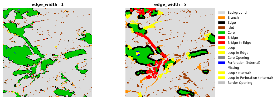
With wider edges, narrow patches have no core left: they turn into bridges, loops, branches and islets, and the core shrinks to the interior of the larger patches.
Other options
| Option | Default | Meaning |
|---|---|---|
connectivity |
8 | 8: pixels touching by a corner belong to the same patch; 4: only by a side |
edge_width |
1 | width of edges and perforations, in pixels |
transition |
True | loops and bridges that cross an edge are drawn in their own colours (changes only the colour table) |
internal |
True | features inside holes of a core get +100, and holes are labelled core-opening (100) or border-opening (220) |
The full list of class codes is in ls.MSPA_CLASSES:
Save and display
ls.write_raster(morph, "forest_mspa.tif")   # GeoTIFF with the MSPA colour table
ls.save(stats, "forest_mspa_stats.csv")      # the table
To draw the classes with their colours in Python, use the show_classes
helper of core concepts with
ls.mspa_colormap().
Simplified pattern analysis (SPA)
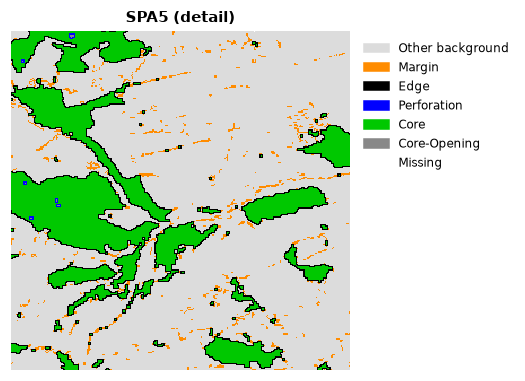
When the seven MSPA classes are more than you need, SPA summarises the pattern in 2, 3, 5 or 6 classes, from "habitat that has a core vs. small linear features" (SPA2) to a split close to MSPA (SPA6):
| Variant | Classes |
|---|---|
| SPA2 | contiguous (core, edge, perforation), small linear features |
| SPA3 | core, edge (+ perforation), margin |
| SPA5 | core, edge, perforation, margin |
| SPA6 | core, edge, perforation, margin, islet |
spa.map is the class map (ls.SPA_CLASSES names the codes), spa.stats
the class areas and spa.porosity the ratio of the core-openings to the
core area. print(spa.summary()) gives a full report.
Objects by size: accounting
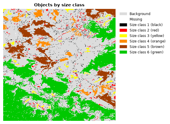
Accounting finds every separate habitat object (a group of connected habitat pixels) and groups them into size classes. It answers questions like "how much of the forest is in large, intact blocks and how much in fragments?".
acc = ls.accounting(forest, thresholds=(50, 250, 1000, 5000, 20000))
ls.plot(acc)          # the size classes, their chart and numbers
acc.stats
The thresholds are the upper sizes of the classes, in pixels: objects of 1 to 50 pixels are class 1, 51 to 250 class 2, and so on; objects above the last threshold are the last class. In the example, 94% of the objects are tiny but they hold less than 5% of the forest, while three objects hold 64% of it.
The result also has:
| Attribute | Content |
|---|---|
acc.classes |
map of size classes (colours: ls.accounting_colormap()) |
acc.ids |
map of object numbers |
acc.area |
map where every object pixel holds the area of its object |
acc.object_area |
area of every object |
acc.largest |
the three largest objects |
acc.summary() |
a printable report, with hectares for a given pixel_resolution |
thresholds="auto" proposes classes from the range of object sizes, and
highlight_largest=True marks the three largest objects on the map.
Parcels: how divided is the landscape?
Parcellation treats every connected region of the same value (habitat or background) as a parcel and measures how finely the landscape is cut:
| Column | Meaning |
|---|---|
Count |
number of parcels of the class |
APS |
average parcel size, pixels |
AWAPS |
area-weighted average parcel size: the size of the parcel a random pixel falls in |
DIVISION |
probability that two random pixels of the class are in different parcels (0 = one parcel, 1 = infinitely divided) |
PARC |
degree of parcellation, % |
parcels.global_stats holds the same values for the whole landscape, and
ls.parcellation(forest, return_labels=True).parcel_labels a map of the
parcels.
Contortion: how convoluted are the boundaries?
Contortion measures how much the boundary of each habitat object bends, relative to its size: compact objects score low, elongated or dendritic ones high.
Values: 0 missing, 1 background, 2 objects that were left out (smaller than
min_area or without an interior), 3 and more the contortion of each
object.
Next steps
- Measure fragmentation at different observation scales in the fragmentation tutorial.
- Process many maps or maps larger than memory with MSPA in large data & batch.
- Every function and option: API reference.