Chapter 12.2

Key concepts¶

Every prioritization, from a small watershed to a continent, is built from the same handful of ingredients. Once they are clear, any planning problem can be read as a list of answers to five questions, and any script of ls.prioritize as the same list written in code.

In this chapter

planning units, features, costs, targets and decisions;
Serra Verde, the example region used in this part of the course;
how a problem is written with ls.prioritize, one ingredient at a time.

Ingredient	The question it answers	In `ls.prioritize`
Planning units	Into which pieces is the landscape divided?	the cells of the cost raster, polygons, H3 cells or table rows
Features	What should be conserved?	one raster (or column) per species, habitat or service
Cost	What does it take to conserve each piece?	the values of the cost raster or column
Targets	How much of each feature is enough?	`add_relative_targets`, `add_absolute_targets`, `add_manual_targets`, ...
Decisions	What can be done with each piece?	`add_binary_decisions`, `add_proportion_decisions`, ...

Serra Verde¶

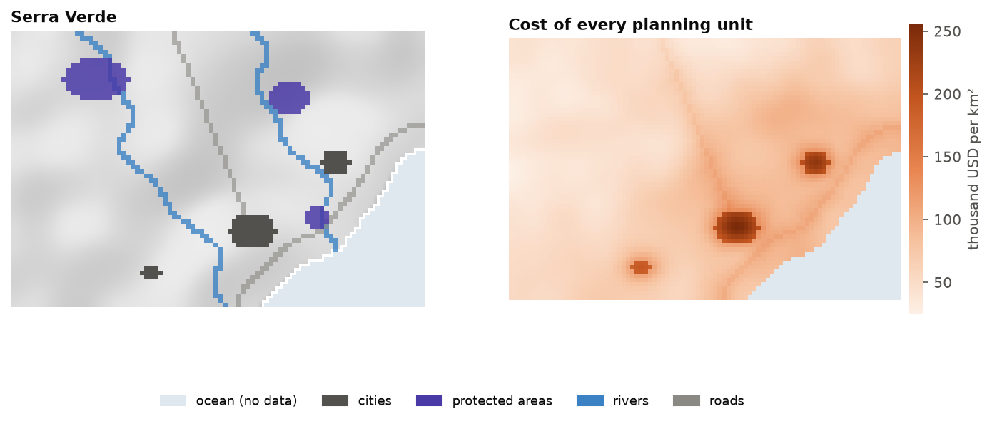
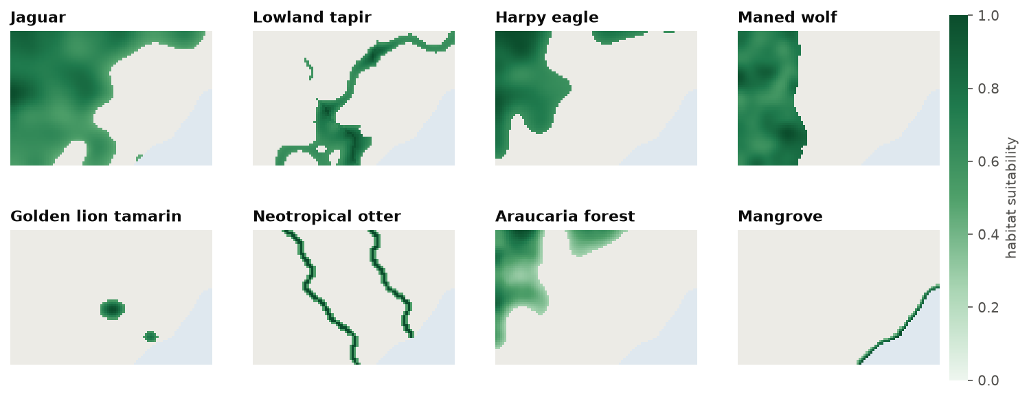
The examples of these chapters use Serra Verde, an imaginary coastal region that ships with Landschaft (ls.prioritize.example_data). It is synthetic, but built to behave like real planning data: mountains in the north-west where land is cheap, a coastal plain with three cities, a highway and two rivers where land is dear, eight features from widespread to very rare, three protected areas, maps of habitat condition, carbon and two threats.

import numpy as np
import landschaft as ls

P = ls.prioritize
cost = ls.load_raster(P.example_data("cost"))
features = ls.load_raster(P.example_data("features"))
print(cost.shape, "cells;", int(np.isfinite(cost.values).sum()), "planning units")
[str(b) for b in features.band.values]

Serra Verde and its costs — Serra Verde: 60 x 90 cells of 1 km. The ocean (south-east) has no cost and is not part of the problem, which leaves 4825 planning units. Land costs from 25 to 256 thousand USD per km²: cheap in the mountains, dear around the cities and along the roads.

Planning units¶

To decide where, the landscape is first cut into pieces. Each piece is a planning unit: the smallest area that can be selected or not. Planning units can be grid cells, properties, watersheds, municipalities or hexagons. In ls.prioritize they are:

the cells of a raster with a cost (cells without a value, NaN, are not planning units: the ocean of Serra Verde);
polygons of a vector layer (problem(polygons, features, cost_column="cost")): the amounts of the features in every polygon are computed exactly from the rasters, cell fractions included;
H3 hexagons (h3_units), an equal-area grid that suits regional and global problems;
the rows of a table, when the amounts are already known per unit.

The size of the units is a trade-off (chapter 2 discusses grain in general):

smaller units describe the landscape more precisely, but make the problem larger, and may give plans too detailed to implement;
larger units are faster and closer to how land is managed (a property, a watershed), but mix good and poor areas in the same unit.

Rule of thumb

Use the resolution at which decisions will be implemented, and no finer than the resolution of the biodiversity data. National plans often use cells of 1 to 10 km; municipal plans 100 m to 1 km. Chapter 12.9 shows how to solve a fine problem on coarser blocks when it is too large.

Features¶

Features are what the plan should conserve:

species: the modelled distribution or habitat suitability of a jaguar, a tree, a frog (chapter 13 explains how such maps are made);
ecosystems and habitats: mangroves, grasslands, old-growth forest;
ecosystem services: carbon, water provision, pollination;
anything with a spatial amount: cultural sites, spawning grounds, climate refugia.

Each feature is a map in which every planning unit holds an amount: presence (1) or absence (0), a probability or suitability between 0 and 1, a number of individuals, tonnes of carbon.

The eight features of Serra Verde — Habitat suitability of the eight features. The jaguar and the maned wolf are widespread; the golden lion tamarin lives in two small lowland forest fragments and the mangrove in a thin coastal strip. Rare features have few places where they can be conserved, and they usually drive the shape of a plan.

Cost¶

Conservation is never free. The cost of a planning unit says what it takes to include it:

acquisition: the price of the land;
opportunity cost: the income lost by not farming, logging or fishing there (Naidoo et al. 2006);
management: patrols, fences, restoration, every year;
area: with no cost data, the area of each unit (a constant for a grid) makes the plan as small as possible.

Cost is what makes the problem interesting. Without it, the best plan would be to protect everything; with it, the question becomes which places give the most for what they cost.

Cost and missing values

The cost raster also says which cells are planning units: cells without a value are left out. A cost of zero is a valid planning unit that costs nothing, and the solver will happily select it. Use missing values for "not part of the problem", and zero only for "free".

Targets¶

A target says how much of each feature is enough:

relative: a share of the feature's total amount, 0.3 for 30 %;
absolute: an amount in the units of the feature, 500 km² of habitat, 2 million tonnes of carbon;
manual: per feature, with a sense (>=, <= or =), for instance at most a given amount of an invasive species;
log-linear: a share that falls as the feature's range grows (Rodrigues et al. 2004): high for rare species, low for widespread ones;
sub-regional: a target inside every region, for instance 30 % of each species in each state.

p = P.problem(cost, features)
p.add_relative_targets(0.3)                                           # 30 % of every feature
p.add_relative_targets([0.3, 0.3, 0.3, 0.3, 0.6, 0.3, 0.3, 0.6])      # more of the rare ones
p.add_loglinear_targets(10, 0.9, 2000, 0.2)                           # 90 % up to a total of 10, 20 % from 2000

Where do targets come from? From policy (protecting 30 % of land and sea by 2030, Target 3 of the Kunming-Montreal Global Biodiversity Framework), from ecology (the area a viable population needs), or from the people involved. Chapter 12.4 shows how the choice changes the plan and its price.

Decisions¶

What can be done with each planning unit? The decision type says it:

binary (add_binary_decisions): a unit is selected (1) or not (0), the usual case for reserves;
proportion (add_proportion_decisions): any share of a unit, for instance "restore 40 % of this cell", when units are large and actions can apply to part of them;
semi-continuous (add_semicontinuous_decisions): any share up to a limit.

Existing reserves and places that cannot be used enter as locked units: add_locked_in_constraints (always selected) and add_locked_out_constraints (never). When the decision is not "in or out" but which action against which threat, the problem becomes a multi-action plan.

Putting it together¶

A problem is written by adding ingredients, one method each, all starting with add_. Every method returns a new problem and leaves the old one untouched, so variants (other targets, other costs) are cheap to make and compare, and the order of the calls does not matter:

protected = ls.load_raster(P.example_data("protected"))
p = (P.problem(cost, features)
       .add_min_set_objective()              # the objective: next chapters
       .add_relative_targets(0.3)            # targets
       .add_locked_in_constraints(protected) # what is already protected
       .add_binary_decisions())              # decisions
sol = p.solve()
sol.status, round(sol.cost), int(sol.values.sum())

sol.coverage[["feature", "relative_target", "relative_held", "met"]].round(3)

The coverage table is the first thing to read after any solve: for every target, how much the plan holds and whether it is met. The one ingredient not discussed yet is the objective: whether to meet every target at the least cost, or to do the most with a fixed budget. That is the subject of chapter 12.4; before it, chapter 12.3 shows the other great family of methods, which does without targets at all.

Key points

Planning units, features, costs, targets and decisions are the five answers every plan needs.
Missing cost values leave cells out of the problem; zero costs make them free.
Targets can be relative, absolute, per feature, log-linear or per region.
A problem is built by adding ingredients; each addition gives a new problem.

References¶

Naidoo, R., Balmford, A., Ferraro, P. J., Polasky, S., Ricketts, T. H., & Rouget, M. (2006). Integrating economic costs into conservation planning. Trends in Ecology & Evolution, 21(12), 681–687.
Rodrigues, A. S. L., Akçakaya, H. R., Andelman, S. J., Bakarr, M. I., Boitani, L., Brooks, T. M., et al. (2004). Global gap analysis: priority regions for expanding the global protected-area network. BioScience, 54(12), 1092–1100.