Chapter 12.5

Spatial design

A plan that meets every target on paper can still fail on the ground if it is a scatter of tiny, isolated cells. This chapter explains why the shape of a plan matters, and the tools ls.prioritize offers to control it: penalties that make plans compact or connected, and constraints that force neighbours, contiguity or corridors.

In this chapter

• why fragmented plans fail, and the "salt and pepper" problem;
• boundary penalties: what the penalty value means and how compactness trades against cost;
• neighbours, contiguity and corridors as hard rules;
• connectivity beyond adjacency: dispersal, rivers and least-cost distances;
• choosing between penalties and constraints.

The salt and pepper problem

Left alone, the solver has no reason to put selected cells next to each other. If two isolated cells are a little cheaper than two neighbouring ones, it takes the isolated ones. On a detailed grid this gives plans that look like salt and pepper sprinkled on the map.

Fragmented plans are a problem because of:

• edge effects: small patches are exposed on every side to wind, fire, invasive species, hunting and noise, and their interior habitat degrades (chapter 3);
• viability: many species need large, continuous areas to keep viable populations;
• management: every separate patch needs its own fences, patrols and negotiations with neighbours. Twenty small reserves cost far more to run than one large one;
• movement: animals and plants must move between patches, more so as the climate changes (chapter 6).

The shape of habitat was the subject of chapter 4; the same measures apply to a plan, and chapter 12.7 shows how to compute them.

Boundary penalties

The most common remedy is the boundary penalty, Marxan's boundary length modifier (BLM; Ball et al. 2009). It adds to the objective a value proportional to the plan's boundary: the length of the edges between selected and unselected cells. Compact plans have short boundaries for the area they cover, so the solver is pulled towards them.

import numpy as np
import landschaft as ls

P = ls.prioritize
cost = ls.load_raster(P.example_data("cost"))
features = ls.load_raster(P.example_data("features"))
p = P.problem(cost, features).add_min_set_objective().add_relative_targets(0.3).add_binary_decisions()

for penalty in (0, 0.002, 0.01, 0.05):
    q = p if penalty == 0 else p.add_boundary_penalties(penalty)
    s = q.add_highs_solver(gap=0.02).solve()
    km = P.eval_boundary_summary(p, s)["boundary"].iloc[0] / 1000
    print(f"penalty {penalty:<6} cost {s.cost / 1000:5.1f} million USD   boundary {km:4.0f} km   "
          f"objective {s.objective:,.0f}")

The 30 % minimum set of Serra Verde with four boundary penalties. As the penalty grows, scattered cells disappear and the plan gathers into a few compact blocks. The chart shows the trade-off: the boundary falls from about 490 km to 225 km, less than half, while the cost rises from 37.2 to 40.0 million USD, about 8 %.

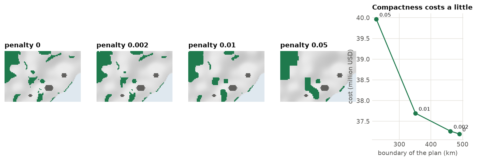
Three things to notice:

1. The objective is no longer the cost. It now includes the penalty times the boundary. Report the cost (s.cost) and the boundary (eval_boundary_summary) separately.
2. The first steps are cheap. The first penalties remove a lot of boundary for little money; past a point, each extra bit of compactness gets expensive. A good value usually lies near the knee of the curve. Chapter 12.6 shows how to find it objectively.
3. The penalty has units. Here cost is in thousand USD and boundary in metres, so a penalty of 0.01 means "I would pay 10 USD to avoid one metre of boundary", 10 000 USD per km. With other data, useful values are very different. That is why the value must be calibrated, never copied from another study.

In plain words

The boundary penalty is a tax on the plan's outline. Every metre of edge between protected and unprotected land costs something. A plan of a few round blocks pays little tax; a plan of a thousand scattered cells pays a lot. The higher the tax, the rounder the plan, and the more it may cost in land.

What is edge_factor?

Cells on the edge of the study area (along the coast, here) have sides that touch no other planning unit. add_boundary_penalties(penalty, edge_factor=0.5) counts those sides at half their length. Use edge_factor=0 when the edge of the study area is not a real edge (a political border across continuous forest), and 1 when it is (a coastline).

Rules on the shape of the plan

Penalties are preferences: the plan may stay fragmented if compactness would be too dear. Sometimes the shape is a rule. ls.prioritize has three kinds of spatial constraints:

Constraint	What it requires
add_neighbors_constraints(k)	every selected unit has at least k selected neighbours: no isolated cells
add_contiguity_constraints()	all selected units form one connected network
add_feature_contiguity_constraints()	the units counted for each feature form one connected network, a network per feature
add_corridor_constraints(terminals, resistance)	given areas (parks, say) are selected and joined by selected units, through low resistance

Hard constraints guarantee the shape you ask for, but they make the problem much harder to solve. Each adds many variables and rows (a flow through the network, for contiguity and corridors). The examples below therefore use Serra Verde on blocks of 3 x 3 km (coarsen, chapter 12.9) and a 20 % target:

c, f = P.coarsen(cost, features, 3)
base = P.problem(c, f).add_min_set_objective().add_relative_targets(0.2).add_binary_decisions()

plain = base.add_highs_solver(gap=0.01).solve()
neigh = base.add_neighbors_constraints(2).add_highs_solver(gap=0.01, time_limit=60).solve()
print(f"no rule: {plain.cost:,.0f}   at least 2 neighbours: {neigh.cost:,.0f}")

# one network, and a corridor between the two mountain parks: each takes from tens of seconds to a minute
contig = base.add_contiguity_constraints().add_highs_solver(gap=0.05, time_limit=120).solve()
terminals = ...   # a raster on the blocks' grid, 1 in the two parks (see the figure script)
corr = base.add_corridor_constraints(terminals, resistance=c).add_highs_solver(gap=0.05, time_limit=120).solve()

The same problem on 3 km blocks under four rules. No rule: scattered blocks. At least two selected neighbours: no block stands alone, but the plan stays in several pieces. One contiguous network: a single winding network that reaches every feature, at a much higher cost. A corridor between the parks (purple): the parks are linked by a chain of cheap blocks, and the rest of the plan stays free.

On these blocks the cost grows from 24.9 million USD with no rule to 27.8 with two neighbours and 31.7 with a single network. Contiguity is the most demanding rule. Here two minutes give a network but do not prove it is the cheapest: its cost is within 17 % of the bound (Gurobi, in ten minutes, finds a network of 30.3 and proves it within 4 %). It is practical for small problems, or when the features lie close to each other. For a whole region, prefer penalties, and use corridors between a few terminals.

Connectivity beyond adjacency

Two areas do not need to touch to be connected. Birds fly, seeds float down rivers, fish swim between reefs. When you know how a feature moves, a connectivity matrix (how strongly each pair of planning units is linked) brings it into the plan:

• add_connectivity_penalties(penalty, data) rewards selecting strongly connected pairs together;
• add_asym_connectivity_penalties(penalty, data) penalizes breaking one-way links, such as a river reach upstream of a selected one (Hermoso et al. 2011);
• in multi-action plans, add_directional_dependencies makes the benefit of an action downstream depend on what is done upstream (chapter 12.8).

The matrices come from simple helpers, or from the connectivity tools of earlier chapters:

Helper	Connectivity
adjacency_matrix(x)	1 between units that touch
boundary_matrix(x)	the length of the boundary they share (what the boundary penalty uses)
connectivity_matrix(x, y)	shared boundary times the mean of a raster y, such as habitat quality
proximity_matrix(x, distance)	1 between units closer than a distance
decay_connectivity(distances, median)	a dispersal probability that halves every median metres, from any distances: Euclidean, least-cost (ls.cost, chapter 9) or resistance distances (ls.circuit, chapter 8)

For example, connectivity through the habitat of the lowland tapir, which follows the rivers:

cm = P.connectivity_matrix(c, f.sel(band="lowland_tapir"))    # shared edge x mean tapir habitat
q = base.add_connectivity_penalties(0.005, cm).add_highs_solver(gap=0.02).solve()
before = P.eval_connectivity_summary(base, plain, cm)["connectivity"].iloc[0]
after = P.eval_connectivity_summary(base, q, cm)["connectivity"].iloc[0]
print(f"cost {plain.cost:,.0f} -> {q.cost:,.0f};  tapir connectivity {before:,.0f} -> {after:,.0f}")

With a penalty of 0.005, the plan keeps pairs of blocks along the tapir's rivers together: the connectivity inside the plan almost doubles (from 0.43 to 0.81 million) for about 1 % more cost. A penalty four times larger triples it again, but makes the plan 45 % dearer: like the boundary penalty, this one needs calibration.

Penalties and their sign

A connectivity penalty in prioritizr's sense is a reward: a positive value makes connected pairs more attractive. The boundary penalty, on the other hand, makes fragmented plans less attractive. In both cases the value is an exchange rate between the units of cost and of the matrix, and it must be calibrated.

Penalties or constraints?

	Penalties (boundary, connectivity, linear)	Constraints (neighbours, contiguity, corridors)
What they guarantee	nothing: a preference, paid for in the objective	the shape, exactly
What they need	a value to calibrate	no value, but a clear rule
Cost to solve	moderate: Landschaft's engines handle them on large maps	high: practical on hundreds to a few thousand units
When	almost always, to avoid salt and pepper	when the rule is a requirement: a corridor between parks, no isolated cells

A good practice is to start without spatial rules, look at the plan, then add a boundary penalty calibrated on the knee of the trade-off, and constraints only where a rule is truly needed.

Key points

• Without spatial terms, plans fragment: edges, viability, management and movement all suffer.
• A boundary penalty is a tax on the plan's outline; its value has units and must be calibrated.
• The first steps of compactness are cheap; the last are expensive.
• Neighbour, contiguity and corridor constraints force a shape, at a price in cost and solving time.
• Connectivity matrices bring dispersal, rivers and least-cost distances into the plan.

Check your understanding

1. A colleague used a boundary penalty of 0.5 in a study with costs in USD and boundaries in km. Can you use the same value with costs in thousand USD and boundaries in metres?
2. Why does a plan with at least two neighbours per cell still come in several pieces?
3. A water agency wants to protect river reaches, and knows that pollution flows downstream. Which tool expresses this?

Answers

1. No. Their 0.5 USD per km is 0.5 / 1000 thousand USD per 1000 m, that is 5 × 10^-7 in your units. Better still, calibrate it anew: the right value also depends on the landscape.
2. The rule is local: each cell needs neighbours, but a group of three cells satisfies it on its own. Only contiguity constraints join all groups into one network.
3. Asymmetric connectivity penalties (a matrix from upstream to downstream reaches), or, with management actions, directional dependencies.

References

• Ball, I. R., Possingham, H. P., & Watts, M. E. (2009). Marxan and relatives: software for spatial conservation prioritization. In A. Moilanen, K. A. Wilson & H. P. Possingham (Eds.), Spatial Conservation Prioritization (pp. 185–195). Oxford University Press.
• Beger, M., Linke, S., Watts, M., Game, E., Treml, E., Ball, I., & Possingham, H. P. (2010). Incorporating asymmetric connectivity into spatial decision making for conservation. Conservation Letters, 3(5), 359–368.
• Hermoso, V., Linke, S., Prenda, J., & Possingham, H. P. (2011). Addressing longitudinal connectivity in the systematic conservation planning of fresh waters. Freshwater Biology, 56(1), 57–70.
• Önal, H., & Briers, R. A. (2006). Optimal selection of a connected reserve network. Operations Research, 54(2), 379–388.
• Stewart, R. R., & Possingham, H. P. (2005). Efficiency, costs and trade-offs in marine reserve system design. Environmental Modeling & Assessment, 10(3), 203–213.
• Williams, J. C., ReVelle, C. S., & Levin, S. A. (2005). Spatial attributes and reserve design models: a review. Environmental Modeling & Assessment, 10(3), 163–181.