Chapter 12.7

Evaluating a plan

A solution is not the end of an analysis. It is a proposal to check: does it meet the targets, by how much, at what cost, in what shape? Which of its places are essential, and which could be swapped for others? This chapter covers the evaluation tools of ls.prioritize. All of them work on any plan, whether it came from the solver, from Zonation, or was drawn by hand in a workshop.

In this chapter

• the summaries to read after every solve: units, cost, boundary, representation, targets;
• importance: replacement cost, irreplaceability, rarity-weighted richness, rank importance and selection frequency;
• the shape of a plan with landscape metrics and MSPA;
• extinction risk;
• a complete report, as a web page.

The first look

Every evaluation function takes the problem and a solution, and returns a table:

import numpy as np
import pandas as pd
import landschaft as ls

P = ls.prioritize
cost = ls.load_raster(P.example_data("cost"))
features = ls.load_raster(P.example_data("features"))
p = (P.problem(cost, features).add_min_set_objective().add_relative_targets(0.3)
       .add_binary_decisions().add_highs_solver(gap=0.001))
sol = p.solve()

pd.concat([P.eval_n_summary(p, sol), P.eval_cost_summary(p, sol)["cost"],
           P.eval_boundary_summary(p, sol)["boundary"]], axis=1)

P.eval_target_coverage_summary(p, sol)[["feature", "met", "relative_target", "relative_held",
                                        "relative_shortfall"]].round(3)

The target coverage says, for every target, whether it is met and by how much. With a minimum set every target is met, and most only just: the solver buys no more than needed. A feature well above its target (here the araucaria forest, at 60 % for a target of 30 %, and the harpy eagle, at 44 %) comes "for free" with the others. It lives where the plan must go anyway.

eval_feature_representation_summary gives the same for every feature, with or without targets, which is what you need to compare plans made with different objectives. The figures of chapter 12.1 and 12.4 are bar charts of it.

Evaluate any plan

The solution argument can be a Solution, a raster of 0/1 (or shares) on the planning units' grid, a table with a solution column, or an array. A park agency's own proposal, a plan from another tool or the existing reserves can all be evaluated against the same problem: P.eval_target_coverage_summary(p, protected) is a gap analysis.

Which places matter most?

A plan of 800 cells is a long list. Stakeholders ask which cells are essential and which could be swapped: importance scores rank the selected units. They answer slightly different questions:

Measure	Question	Cost
eval_replacement_importance (Cabeza & Moilanen 2006)	how much dearer does the plan get if this unit is lost and the rest re-optimized?	one solve per selected unit
eval_ferrier_importance (Ferrier et al. 2000)	how likely is this unit to be needed to meet the targets, over all plans of the same size?	instant
eval_rare_richness_importance (Albuquerque & Beier 2015)	how much rare biodiversity does this unit hold?	instant
eval_rank_importance (Jung et al. 2021)	how early does this unit enter the plan as the budget grows?	a few solves
portfolio selection frequency (12.6)	in how many near-optimal plans does this unit appear?	one portfolio

rc = P.eval_replacement_importance(p, sol)            # rescaled from 0.01 to 1
fe = P.eval_ferrier_importance(p, sol)                 # one band per feature, plus "total"
rw = P.eval_rare_richness_importance(p, sol)
port = p.add_highs_solver(gap=0.01).add_gap_portfolio(20, pool_gap=0.02).solve()

sel = sol.selection.values > 0.5
scores = pd.DataFrame({"replacement": rc.values[sel], "ferrier": fe.sel(band="total").values[sel],
                       "rarity": rw.values[sel], "frequency": port.frequency.values[sel]})
scores.corr(method="spearman").round(2)

Three views of the importance of the cells of Serra Verde's 30 % plan. Replacement cost (left) and Ferrier's irreplaceability (middle) are highest in the tamarin's lowland fragments and the mangrove, which have no substitutes. Right: in 20 plans within 2 % of the optimum, most cells are always selected, while a few cells in the mountains swap places from one plan to the next.

In plain words

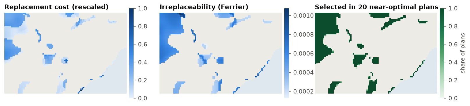
Replacement cost is the price of losing a cell: if a landowner refuses, how much more will the rest of the plan cost? Irreplaceability is the chance the cell is needed: if it holds the only habitat left of a species, it is needed in every plan. Selection frequency is a vote among good plans. The three usually agree on the essential cells and disagree on the ordinary ones, which is fine: the ordinary ones are, by definition, interchangeable.

In Serra Verde, Ferrier's irreplaceability and rarity-weighted richness rank the cells much alike (a Spearman correlation of 0.86), and replacement cost agrees with them moderately (0.55). Selection frequency agrees with none of them, and for a simple reason: 794 cells are in all 20 near-optimal plans and only 20 cells vary, so it separates a handful of interchangeable cells from the rest. It is most informative when the portfolio is wider (a larger pool_gap) or the problem has many near-ties.

Replacement cost is the most direct, and the slowest: it solves the problem again for every selected unit (in parallel, with the solution as a starting point). Use a small gap, since a gap of 1 % on a 37 million plan is 370 thousand USD of noise, more than the replacement cost of most cells. Ferrier's and rarity scores are instant and work on any plan.

The shape of a plan

A plan is also a landscape: a map of selected and unselected cells. The tools of chapter 5 and chapter 4 describe its shape:

lm = P.eval_landscape_metrics(sol, metric=["np", "area", "enn"])     # families, as in landscapemetrics
lm[["metric", "value"]].round(1)

mspa, areas = P.eval_mspa(sol)
areas

The number of patches (np), their areas and the distance from each to the nearest other patch (enn) say how fragmented the plan is: here 17 patches. MSPA says how much of it is core (far from any edge): 59 % of the plan, with 27 % edge and 6 % islets, cells too small to have a core. Comparing plans with and without a boundary penalty (chapter 12.5) with these measures shows what compactness bought.

Extinction risk

Targets say whether a plan reaches a threshold. The species-area relationship (chapter 12.4) says what a plan is worth for persistence: the risk 1 − (held / total)^z of every feature, and their sum, the expected number of features lost if all habitat outside the plan disappeared.

P.eval_extinction_risk(p, sol).round(3)

It is a coarse model. Real responses to habitat loss vary between species and depend on configuration, not only area. Use it to compare plans, not to predict extinctions.

A complete report

report runs the usual evaluations at once (summary, representation, targets, importance, optionally the extinction risk and a comparison with Zonation) and ls.plot turns them into a web page with maps, charts and tables, to send to colleagues or stakeholders:

r = P.report(p, sol, extinction_z=0.25)
page = ls.plot(r, show=False).save("serra_verde_report.html")

ls.plot also draws any solution, portfolio or trade-off on its own: ls.plot(sol) opens an interactive map, ls.plot(port) the selection frequency, ls.plot(cal) the calibration curve.

A checklist

Before presenting a plan, check:

1. status and gap: "optimal" and a small gap, or a reason why not;
2. targets: all met, and which ones are far above their target (and why);
3. cost: in the units of the cost layer, with the penalty terms reported apart from it;
4. shape: the number and size of patches, and whether isolated cells make sense on the ground;
5. importance: the essential places, and the flexible ones;
6. alternatives: a portfolio or scenarios, to show that other choices exist;
7. data: the features and costs that drive the result, and how certain they are.

Key points

• Read the target coverage after every solve; features far above target come "for free".
• The evaluation functions work on any plan: solutions, existing reserves, hand-drawn proposals.
• Replacement cost, irreplaceability and selection frequency agree on essential places and disagree on interchangeable ones.
• Landscape metrics and MSPA describe a plan's shape; extinction risk its value for persistence.
• report and ls.plot package all of it for others.

Check your understanding

1. A cell has a replacement cost of zero. What does this mean?
2. Why use a small gap when computing replacement costs?
3. How would you do a gap analysis of Serra Verde's existing protected areas?

Answers

1. Without it, the solver finds another plan of the same cost: an equally good substitute exists.
2. Each replacement cost is the difference between two optimized costs. If each is only known to within 1 %, the difference is mostly noise for cells whose real replacement cost is small.
3. Load the protected areas as a raster (P.example_data("protected")) and evaluate it as a solution: P.eval_target_coverage_summary(p, protected) gives how much of every target they already meet.

References

• Albuquerque, F., & Beier, P. (2015). Rarity-weighted richness: a simple and reliable alternative to integer programming and heuristic algorithms for minimum set and maximum coverage problems in conservation planning. PLoS ONE, 10(3), e0119905.
• Baisero, D., Schuster, R., & Plumptre, A. J. (2022). Redefining and mapping global irreplaceability. Conservation Biology, 36(2), e13806.
• Cabeza, M., & Moilanen, A. (2006). Replacement cost: a practical measure of site value for cost-effective reserve planning. Biological Conservation, 132(3), 336–342.
• Ferrier, S., Pressey, R. L., & Barrett, T. W. (2000). A new predictor of the irreplaceability of areas for achieving a conservation goal, its application to real-world planning, and a research agenda for further refinement. Biological Conservation, 93(3), 303–325.
• Jung, M., Arnell, A., de Lamo, X., García-Rangel, S., Lewis, M., Mark, J., et al. (2021). Areas of global importance for conserving terrestrial biodiversity, carbon and water. Nature Ecology & Evolution, 5, 1499–1509.
• Soille, P., & Vogt, P. (2009). Morphological segmentation of binary patterns. Pattern Recognition Letters, 30(4), 456–459.