Routes on grids

Many questions about movement come down to one: how hard is it to go from here to there across this landscape? A hiker climbs slowly and descends fast; an animal avoids open ground; people spread along coasts and valleys. Seen as a graph, a raster answers these questions: every cell is a node, neighbouring cells are joined, and each connection carries a conductance, how easily it is crossed. Least-cost distances, cost surfaces, the route a walker would take, how much two routes share: all are computed on that graph.

You will learn to:

• build the graph of a raster (a transition) from any rule of the two cells' values, including direction-dependent ones;
• compute travel-time surfaces, least-cost distances and paths;
• go from the single best route to the whole bundle of likely routes, with random walks and randomised shortest paths;
• measure how much routes from a common origin overlap, and relate that to genetic distances between populations.

Everything lives in ls.cost. The results match the R package gdistance, value for value where the arithmetic allows (transitions, cost distances and paths) and to about 1e-12 where sparse linear systems are solved.

A transition: the raster as a graph

ls.cost.transition connects every pair of neighbouring cells (4, 8 or 16 directions) that both have a value, with a function of the two values. The connection's value is a conductance: large means easy.

import numpy as np
import landschaft as ls

resistance = np.array([[1.0, 1.0, 4.0],
                       [1.0, 9.0, 4.0],
                       [1.0, 1.0, 1.0]])
tr = 1 / ls.cost.transition(resistance, "mean", 8)     # conductance = 1 / mean resistance
tr = ls.cost.geo_correction(tr)                        # / distance between cell centres
print(tr)

Transition(3 x 3 cells, 8 directions, symmetric, conductance, 40 connections)

geo_correction divides every conductance by the distance between the two cell centres, so that diagonal steps cost more than straight ones; on longitude/latitude grids it uses distances on the ellipsoid. A symmetric transition has one value per pair; with symmetric=False each direction has its own, which is what slopes need.

Hiking on a volcano

The Maungawhau volcano in Auckland ships as example data (elevation, 10 m cells). Tobler's hiking function gives the walking speed from the slope: about 6 km/h on a gentle descent, slower uphill and on steep descents.

dem = ls.load_raster(ls.cost.example_data("maungawhau"))
rise = ls.cost.transition(dem, "diff", 8, symmetric=False)    # elevation to - elevation from
slope = ls.cost.geo_correction(rise)                          # rise / distance
speed = slope.map(lambda s: 6 * np.exp(-3.5 * np.abs(s + 0.05)) / 3.6, pairs="all")   # m/s
conductance = ls.cost.geo_correction(speed)                   # 1 / seconds per step

map(..., pairs="all") applies the function to every pair of neighbours, also to the flat ones whose rise is 0 (and so had no connection). The cost of a step is the reciprocal of the conductance, here the seconds it takes. From A at the foot of the volcano to B on the other side, and back:

A, B = (2667670, 6479000), (2667800, 6479400)
minutes = ls.cost.cost_distance(conductance, [A, B]) / 60
print(minutes.round(1))

[[0.  7.5]
 [8.1 0. ]]

The two directions differ: the way back climbs where the way out descended. acc_cost gives the travel time from A to every cell, and shortest_path the routes:

time_from_a = ls.cost.acc_cost(conductance, A)
there = ls.cost.shortest_path(conductance, A, B, output="lines")
back = ls.cost.shortest_path(conductance, B, A, output="lines")
ls.plot([(time_from_a / 60).rename("minutes from A"), there, back])   # one map, three layers
ls.write_vector(there, "path_a_to_b.gpkg")
print(round(float(time_from_a.max()) / 60, 1), round(there.length.iloc[0]), round(back.length.iloc[0]))

11.6 487 487

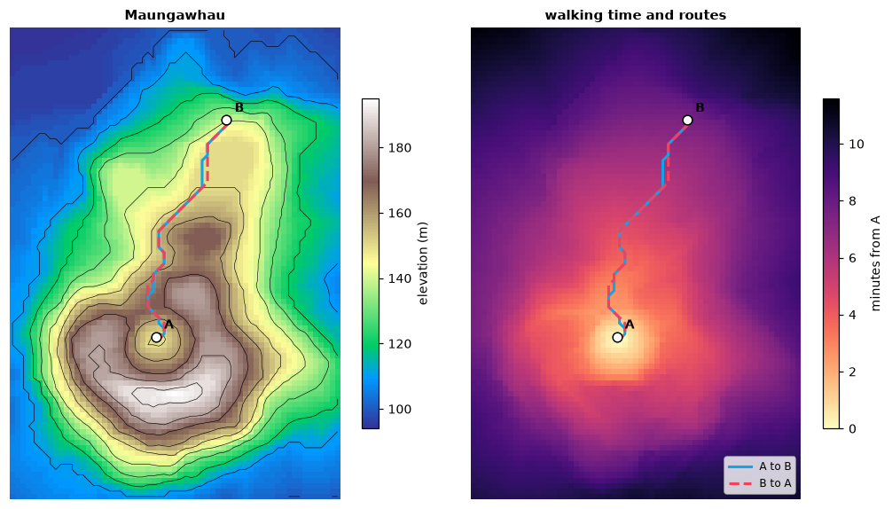
Every cell of the volcano is less than 12 minutes from A. The two routes are equally long (487 m) but take different lines around the crater. cells and transition are the other outputs of shortest_path; among equally cheap paths the function always returns the same one.

From the best route to all likely routes

A least-cost path assumes a walker who knows the whole landscape. A random walk assumes one who knows nothing and steps to a neighbour with a probability proportional to the conductance. Randomised shortest paths sit in between: the parameter theta sets how strongly the walk prefers cheap routes, from the random walk (0) to the least-cost path (large values). passage maps how often the walk from A to B crosses each cell:

routes = {theta: ls.cost.passage(conductance, A, B, theta=theta) for theta in (0, 0.001, 0.01, 1)}
print({theta: round(float((p > 0.01).mean()), 3) for theta, p in routes.items()})

{0: 0.917, 0.001: 0.18, 0.01: 0.118, 1: 0.019}

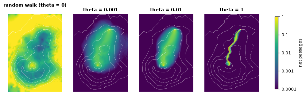
The random walk (theta = 0) passes through 92 % of the volcano's cells more than once in a hundred walks; with theta = 0.001 (per second of walking) 18 %, and with 1 it keeps to a narrow band (2 %) along the least-cost route. The same walks give distances: rsp_distance is the expected cost of the walk, and commute_distance the expected time of a random walk to go and come back (for symmetric transitions: it is the effective resistance of the circuit view, times the sum of all conductances).

print(ls.cost.rsp_distance(conductance, [A], [B], theta=0.1).round(0))
symmetric = ls.cost.geo_correction(1 / ls.cost.transition(dem, "mean", 8))
print(ls.cost.commute_distance(symmetric, [A, B]).round(0))

[[534.]]
[[    0. 35013.]
 [35013.     0.]]

The randomised walk takes 534 s on average, 83 s more than the least-cost route (451 s).

Routes of dispersal from a common origin

If populations spread out from one origin, two populations whose routes share much of the way should be closer genetically than two whose routes split early. The example data hold the genetic distances between 23 European populations of the Y-chromosome haplogroup R1b1b2 and their locations, and a map of Europe (land = 1, 1/3 degree cells).

europe = ls.load_raster(ls.cost.example_data("europe"))
pops = ls.load_table(ls.cost.example_data("pop_coord"))
genetic = ls.load_table(ls.cost.example_data("gen_dist")).set_index("population")
walk = ls.cost.geo_correction(ls.cost.transition(europe, "mean", 16), "r", scale=True)

xy = pops[["x", "y"]].to_numpy()
routes = ls.cost.path_inc(walk, (37.0, 39.0), xy)    # from Anatolia
pairs = np.triu_indices(len(pops), 1)
g = genetic.loc[pops["population"], pops["population"]].to_numpy()[pairs]
print({name: round(float(np.corrcoef(m[pairs], g)[0, 1]), 2) for name, m in routes.items()})

{'overlap': -0.73, 'nonoverlap': 0.56}

path_inc computes, for every population, the flow of a random walk from the origin to it on every connection, then for every pair of populations the flow the two routes share (overlap) and the flow they do not (nonoverlap), each connection weighted by its cost. The more two routes overlap, the smaller the genetic distance (a correlation of -0.73). For comparison:

coast = ls.cost.geo_correction(ls.cost.transition(europe, "mean", 16), "c")
least_cost = ls.cost.cost_distance(coast, xy)
commute = ls.cost.commute_distance(walk, xy)
print(round(float(np.corrcoef(least_cost[pairs], g)[0, 1]), 2),
      round(float(np.corrcoef(commute[pairs], g)[0, 1]), 2))

0.59 -0.03

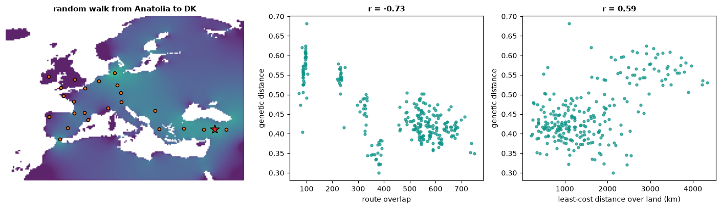
Least-cost distances over land explain less (0.59) and commute distances, which ignore the direction of spread, nothing (-0.03). Correlations between the pairs of one set of points are not independent: test them with a Mantel test (permuting the populations) before drawing conclusions.

Advanced options

• Directions: 16 directions add the knight moves (two cells one way, one the other), which make least-cost routes less angular.
• Longitude/latitude grids: distances between cells are geodesic; on a grid spanning 360 degrees the columns wrap around the 180th meridian. For random walks use geo_correction(tr, "r"), which also shrinks north-south connections towards the poles.
• Any rule: a callable receives the two cells' values (x[0] the first cell, x[1] the second) for all connections at once; map, *, + and numbers combine transitions; normalize gives the random walk's probabilities; sum_reciprocal adds resistances in series.
• Weights for route overlap: path_inc(..., weight=...) takes another transition or a list of them; ls.cost.barriers(r, breaks=[...]) marks the connections that cross given values (or, without breaks, the boundaries between categories) and ls.cost.areas(r) those inside each category, to ask how much of the routes' overlap happens across a barrier or in an area.
• Randomised shortest paths: method=2 in rsp_distance weights the steps by P ** theta instead of exp(-theta * cost) * P; total_net counts every passage instead of the net ones.
• Speed: the graph is never built as a matrix; least-cost searches run directly on the grid, and several sources in parallel. Linear systems are factorised with a nested-dissection sparse Cholesky (4 million cells: a cost surface in 0.6 s, a random-walk passage map in 4.5 s).