Chapter 12.3

Ranking a landscape

A ranking gives every cell of a landscape a priority, from the first to give up to the last. It needs no target and no budget: the best 10 % lies inside the best 30 %, so the same map answers every budget at once, and performance curves tell what each share of the landscape keeps of every feature. This chapter explains how Zonation builds such a ranking (Moilanen et al. 2005, 2022), the method behind ls.prioritize.zonation.

In this chapter

• marginal loss, and the core-area and additive-benefit rules;
• how Zonation 5 sorts a landscape again and again until the order holds;
• reading rank maps and performance curves;
• weights, costs, existing reserves, connectivity, and the limits of the data.

In plain words

Imagine removing the landscape one cell at a time, always the cell whose loss would hurt the features least, given what is still left. The cells left at the end are the irreplaceable core; the order in which the others went is the ranking.

How Zonation ranks

Zonation (Moilanen et al. 2005, 2022) builds the ranking backwards: it removes the cells one after the other, always the one whose removal causes the smallest marginal loss to the features, given the cells still remaining. The last cells remaining are the most important.

Every feature j is first scaled so that its values over the landscape sum to 1: f_ij is the share of feature j in cell i, and R_j the share still remaining. The marginal loss δ_i of cell i combines, over the features, the fraction w_j f_ij / R_j of what remains of each that the cell would take away (w_j is the feature's weight). The rules differ in how they combine them:

Rule	Marginal loss δi	Behaviour
CAZMAX (core-area)	maxj wj fij / Rj	a cell is as valuable as its most important feature; protects the core of every feature's distribution
CAZ1	Σj wj fij / Rj	adds the losses: cells with many features rise
CAZ2 (Zonation 5's default)	√( Σj (wj fij / Rj)² )	between the two: large single losses dominate, several moderate ones still count
ABF (additive benefit)	Σj wj [Rjz − (Rj − fij)z]	the loss of a benefit V(R) = Rz that saturates: the first losses of a feature cost little, the last ones much

CAZMAX, CAZ1 and CAZ2 are one family, the p-norms of the relative losses for p = ∞, 1 and 2 (CAZP takes any p). ABF (Arponen et al. 2005; Moilanen 2007) represents the idea that each feature's benefit grows with the fraction kept, with diminishing returns: with z = 0.25, keeping half of a species gives 84 % of its benefit.

In the four-site example of chapter 12.1, all features start at R_j = 1. Site D holds a third of species 1 and nothing else, so its core-area loss is 1/3; B holds half of species 2 (1/2); A and C each hold all of a species (1). D goes first. Species 1 then has R₁ = 2/3, and B's loss is max((1/3) / (2/3), 1/2) = 0.5: B goes next, and A and C remain. You can check the first step:

import numpy as np
import landschaft as ls

sites = np.array([[1, 1, 0, 1], [1, 1, 0, 0], [1, 0, 0, 0], [0, 0, 1, 0]],
                 dtype="float32")[:, None, :]                       # 4 species x 4 sites
f = sites[:, 0, :] / sites[:, 0, :].sum(axis=1, keepdims=True)   # f_ij
print("CAZMAX losses of A, B, C, D:", f.max(axis=0).round(3))

Recomputing every loss after every removal is slow on maps of millions of cells. Zonation 5 turns the problem around: given an order of removal, the remaining share of every feature when each cell goes is known, and so is every cell's loss at that point. Sorting the cells by these losses gives a new order; Zonation repeats until the order stops changing (the mean ranking error falls below 0.01 %), usually after tens to a few hundred sorts.

Reading the results

The rank map gives every cell a value from 0 (removed first) to almost 1 (the most important). The top fraction of the landscape is a threshold on it: the best 17 % are the cells ranked 0.83 or more.

The performance curves follow every feature as the landscape is removed: at each rank, the share of the feature still in the remaining cells. They answer the practical question: if the best 30 % were protected, how much of each species would it hold? Four species of the CORINE map from the tutorial, each smoothed with a dispersal kernel of about 500 m, so that a cell's value is the habitat around it (see connectivity below):

import pandas as pd
import xarray as xr

clc = ls.load_raster(ls.example_data("clc"))

def share(*codes):
    """The fraction of every 125 m cell covered by the land-cover classes."""
    return clc.isin(codes).coarsen(x=5, y=5).mean().astype("float32")

names = ["forest_bird", "mire_plant", "grassland_butterfly", "farmland_bird"]
species = xr.concat([share(23, 24, 25), share(35, 36), share(18, 26),
                     share(20, 21) + 0.3 * share(12)], dim="species")
res = ls.prioritize.zonation(species, names=names,
                             connectivity=[ls.prioritize.Kernel("negexp", 4)] * 4)   # 4 cells of 125 m

def kept(res, best):
    """The share of every feature in the best `best` fraction of the cells."""
    fc = res.feature_curves
    return fc.iloc[(fc["rank"] - (1 - best)).abs().argmin(), 1:]

pd.DataFrame({"best 17 %": kept(res, 0.17), "best 30 %": kept(res, 0.30)}).round(2)

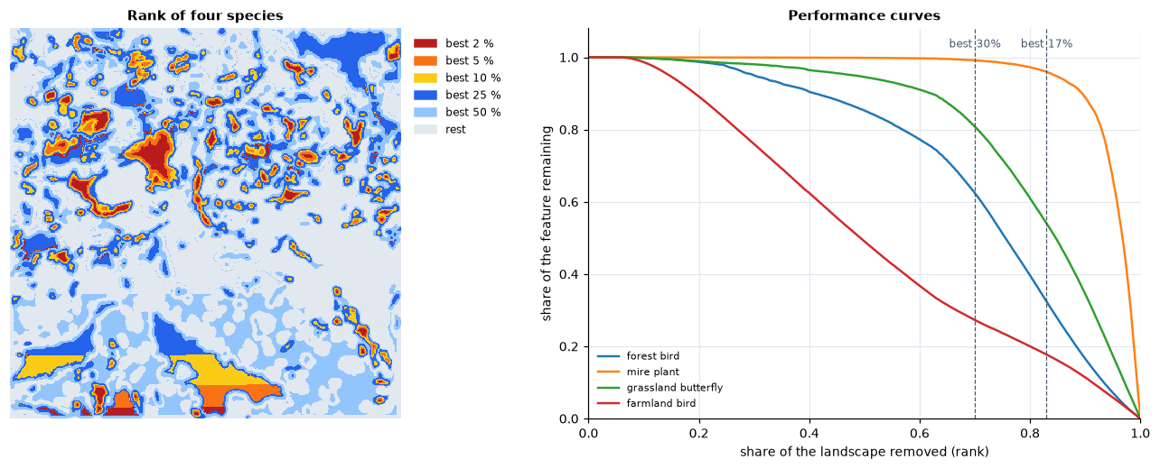
The mire plant, which lives in a few bogs, is almost entirely in the best 17 % (96 %); the grassland butterfly has half of its habitat there (54 %) and 81 % in the best 30 %; the forest bird, spread over a fifth of the map, 32 % and 62 %; the farmland bird, spread thinly over half of the map, a fifth to a quarter (18 % and 27 %). (The straight edges at the bottom of the rank map are ties between cells of equal value; see data and uncertainty.) The curve of a feature falls slowly while cells poor in it are removed, then steeply: its steep part marks where the landscape could not be given up without losing it.

The area percentages echo policy targets: 17 % of land in protected areas (Aichi Target 11, 2010) and 30 % by 2030 (Target 3 of the Kunming-Montreal Global Biodiversity Framework, 2022). A performance curve shows what a given share of land achieves for each feature, which is the substance behind such targets. The area under the mean curve (res.auc) summarises a whole ranking in one number, to compare alternatives.

Weights, costs and what is already protected

Weights say how much a feature matters relative to the others: a threatened species, an endemic one, or one the project is responsible for. They multiply its losses, so its cells are removed later. Negative weights mark features to avoid: a threat, an invasive species, land with conflicting uses.

Costs turn the question into one of efficiency: the marginal loss of a cell is divided by its cost, so cheap cells that hold a little of everything move up (Naidoo et al. 2006). The curves can then be read against the budget instead of the area. Costs can be land prices, management costs, or the opportunity cost of forgone production.

Existing reserves enter as a hierarchic mask: cells of a higher mask level are removed only after all the cells of lower levels, so they rank on top and the rest of the landscape is ranked for what they lack. The share of every feature within the reserves is the gap analysis; the cells ranked just below them are the best extensions.

Connectivity and persistence

A cell of forest surrounded by forest is worth more to a forest species than the same cell alone in a field: populations in large, connected areas persist, those in isolated fragments often do not (chapters 3, 6 and 7). Zonation takes this into account by smoothing each feature with a dispersal kernel before the ranking (Moilanen et al. 2005): every cell receives value from the habitat around it, at the scale the species moves. The ranking then favours compact, connected areas over scattered fragments, at a small cost in raw coverage. Interactions link features to one another (a predator to its prey, a pollinator to its flowers), and the matrix connectivity of Zonation 5 lets features of related habitats count for one another.

Data and uncertainty

A ranking is only as good as the maps it ranks. Some cautions:

• Surrogates. Species distribution models, habitat maps and land-cover classes stand in for the true distributions. Their errors pass into the ranking, unevenly: rare species with few records are the least certain and often the most influential.
• Extent and edges. A species rare in the study area may be common next door; a ranking within administrative borders gives priority to the edge of ranges. Where possible, rank within the ecological context, or weight features by the share of their global range the region holds.
• Resolution. Coarse cells mix habitats and overstate co-occurrence (chapter 2).
• Ties. Cells with exactly the same values have the same marginal loss, and like any sort Zonation orders them by their position (row by row). A map with large uniform areas (every cell of a class worth the same) gets arbitrary stripes in its rank map; ranks within such ties mean nothing. Smoothing with a dispersal kernel, or any more informative feature, breaks them.
• Alternatives. Rankings with different rules, weights, costs or data differ in detail. The robust priorities are those that hold across them; the flexibility map (ZonationResult.flexibility_map) shows how far each cell could move before its loss differs markedly from its neighbours in the order.

Game et al. (2013) review mistakes common in priority setting, among them ignoring costs, confusing high threat with high priority, and ignoring the chance that actions succeed. A ranking says where the landscape is irreplaceable for the features in the analysis; turning it into actions needs the people, institutions and threats of the place.

Key points

• Zonation ranks the whole landscape by removing, again and again, the cells whose loss matters least; the order answers every budget at once.
• The rules differ in how they combine the losses of the features: CAZMAX follows the worst-off feature, ABF the sum of benefits, CAZ2 sits between.
• Performance curves show what any share of land achieves for every feature; weights, costs, reserves and connectivity turn a generic ranking into a plan.
• Rankings inherit the errors of their data: test alternatives and keep the priorities that hold.

Check your understanding

1. A ranking with CAZMAX and one with ABF of the same data give different best 10 %. Which one would you expect to hold more of the rarest species, and which more of the species on average?
2. A region wants to protect 30 % of its land. Why is a ranking useful while the target and budget are still being negotiated?
3. Why do large uniform areas give stripes in a rank map, and how can they be avoided?

Answers

1. CAZMAX keeps the core of every feature, whatever the others do, so it tends to protect more of the rarest; ABF adds benefits over all features and tends to give a higher average coverage, letting a few features fall lower.
2. A ranking is nested: the best 20 %, 30 % or 40 % come from the same map, and the performance curves show what each option achieves for every feature, so the trade-offs of different targets and budgets can be discussed without new analyses.
3. Cells with exactly the same values tie, and ties are broken by position. Smoothing the features with a dispersal kernel (connectivity) or any more informative feature breaks the ties.

References

• Arponen, A., Heikkinen, R. K., Thomas, C. D., & Moilanen, A. (2005). The value of biodiversity in reserve selection: representation, species weighting, and benefit functions. Conservation Biology, 19(6), 2009–2014.
• Game, E. T., Kareiva, P., & Possingham, H. P. (2013). Six common mistakes in conservation priority setting. Conservation Biology, 27(3), 480–485.
• Moilanen, A. (2007). Landscape Zonation, benefit functions and target-based planning: unifying reserve selection strategies. Biological Conservation, 134(4), 571–579.
• Moilanen, A., Franco, A. M. A., Early, R. I., Fox, R., Wintle, B., & Thomas, C. D. (2005). Prioritizing multiple-use landscapes for conservation: methods for large multi-species planning problems. Proceedings of the Royal Society B, 272, 1885–1891.
• Moilanen, A., Lehtinen, P., Kohonen, I., Jalkanen, J., Virtanen, E. A., & Kujala, H. (2022). Novel methods for spatial prioritization with applications in conservation, land use planning and ecological impact avoidance. Methods in Ecology and Evolution, 13(5), 1062–1072.
• Naidoo, R., Balmford, A., Ferraro, P. J., Polasky, S., Ricketts, T. H., & Rouget, M. (2006). Integrating economic costs into conservation planning. Trends in Ecology & Evolution, 21(12), 681–687.