Change detection
Two maps of the same area at two dates: what changed? Beyond counting pixels gained and lost, the tools here separate real structural change from noise at patch boundaries, and describe how fragmentation and the land-use mix shifted.
You will learn to:
- map habitat gains and losses;
- separate structural change from boundary noise, and measure elasticity;
- compare fragmentation classes between dates (transition matrices);
- follow fragmentation at several scales and the land-use mix over time.
Input: two binary habitat maps on the same grid (landscape-mosaic change uses three-class land-cover maps).
We make a second date from the example map by clearing two blocks of forest and planting a new one:
import numpy as np
import landschaft as ls

before = ls.load_raster(ls.example_data("input"))
after = before.copy()
v = after.values
v[600:700, 100:260] = np.where(v[600:700, 100:260] == 2, 1, v[600:700, 100:260])   # clear-cut
v[820:900, 400:560] = np.where(v[820:900, 400:560] == 2, 1, v[820:900, 400:560])   # clear-cut
v[250:330, 420:520] = np.where(v[250:330, 420:520] == 1, 2, v[250:330, 420:520])   # plantation
With real data, load both dates with ls.load_raster and make sure they share
the grid (same size, cell size and extent).
Gains and losses
simple = ls.simple_change(before, after)
ls.plot(simple)       # the change map and its numbers
simple.gain, simple.loss, simple.net_change
Code in simple.change_map |
Meaning |
|---|---|
| 11 | stable background |
| 12 | gain (background → habitat) |
| 21 | loss (habitat → background) |
| 22 | stable habitat |
print(simple.summary()) gives the full report, and ls.write_raster
saves the map with its colour table.
Structural change vs. boundary noise
Two maps made from different images or with different methods rarely agree exactly along patch edges: a band of one or two pixels flips back and forth without any real change. Morphological change detection keeps as real change only what is connected to changes of the patches' interiors, and labels the rest spurious:
mcd = ls.morphological_change(before, after)
ls.save(mcd, "forest_change")      # the change map (GeoTIFF with its colours), tables and numbers
mcd.mcd_gain, mcd.mcd_loss, mcd.spurious, round(mcd.elasticity, 3)
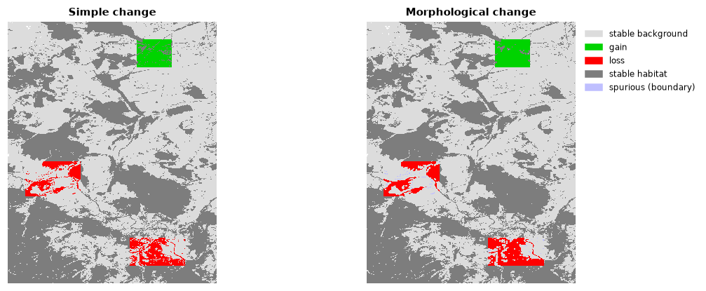
Code 176 in mcd.change_map marks the spurious pixels. Elasticity relates
the total change to the habitat area: a stable landscape has a low value.
Shifts between fragmentation classes
Compute the fragmentation of both dates at the same scale (see the fragmentation tutorial), then compare:
frag_before = ls.fos(before, window_size=27)
frag_after = ls.fos(after, window_size=27)
shift = ls.fos_change(frag_before.map, frag_after.map)
shift.matrix_6x6
The 6 × 6 matrix counts the habitat pixels that moved from each class (rows,
first date) to each class (columns, second date): the diagonal is stable,
above it fragmentation decreased, below it increased.
shift.frag_increase_pct and shift.frag_decrease_pct summarise it and
shift.change_map maps it.
Several scales at once
One transition table per observation scale (7 to 243 pixels) and one for the
multiscale combination, in multi.scales and multi.averages. It accepts
the maps directly (it runs the multiscale density on both) or results of
ls.fad_multiscale.
Change of the land-use mix
With two three-class land-cover maps (1 agriculture, 2 natural, 3 developed),
ls.landscape_mosaic_change(map_2000, map_2020, window_size=27) compares
their landscape-mosaic heat maps: which
compositions became more or less frequent. ls.write_table(table, path) writes it.
Next steps
- Metrics of many dates at once:
SpatioTemporalAnalysisin the landscape metrics tutorial. - Connectivity over time:
ls.conn.eca_changein habitat networks.