Neutral landscapes

A neutral landscape model (NLM) builds a map from a rule and nothing else: cells drawn at random, a gradient, clusters grown from seeds, a fractal surface. Because no ecological process shaped it, an NLM is a null model: comparing a real map, or the result of a simulation on it, with many NLMs tells whether the pattern differs from what chance alone would give.

You will learn to:

• simulate the main families of neutral landscapes;
• turn a continuous model into habitat maps with a chosen habitat share;
• test whether a real map is more aggregated than random ones;
• reproduce landscapes made with the R package NLMR.

All models live in ls.nlm and return an xarray.DataArray on a grid with its origin at (0, 0) and cells of size resolution. Every model takes a seed: the same seed gives the same landscape, and the same landscape as NLMR.

A gallery of models

import numpy as np
import landschaft as ls

models = {
    "random": ls.nlm.random(200, 200, seed=1),
    "planar gradient": ls.nlm.planar_gradient(200, 200, direction=60),
    "edge gradient": ls.nlm.edge_gradient(200, 200, direction=60),
    "distance gradient": ls.nlm.distance_gradient(200, 200, origin=(90, 110, 90, 110), nlmr_compat=False),
    "midpoint displacement": ls.nlm.mpd(200, 200, roughness=0.6, seed=2, nlmr_compat=False),
    "fractional Brownian motion": ls.nlm.fbm(200, 200, fract_dim=1.4, seed=3),
    "Gaussian field": ls.nlm.gaussian_field(200, 200, autocorr_range=20, seed=4),
    "random clusters": ls.nlm.random_cluster(200, 200, p=0.55, ai=[0.3, 0.3, 0.4], seed=5),
    "neighbourhood clusters": ls.nlm.neigh(200, 200, p_neigh=0.95, p_empty=0.002, categories=4, seed=6),
    "rectangular clusters": ls.nlm.random_rectangular_cluster(200, 200, minl=5, maxl=30, seed=7),
    "Voronoi mosaic": ls.nlm.mosaic_tess(200, 200, germs=60, seed=8),
    "Poisson line mosaic": ls.nlm.mosaic_field(200, 200, n=20, seed=9),
}

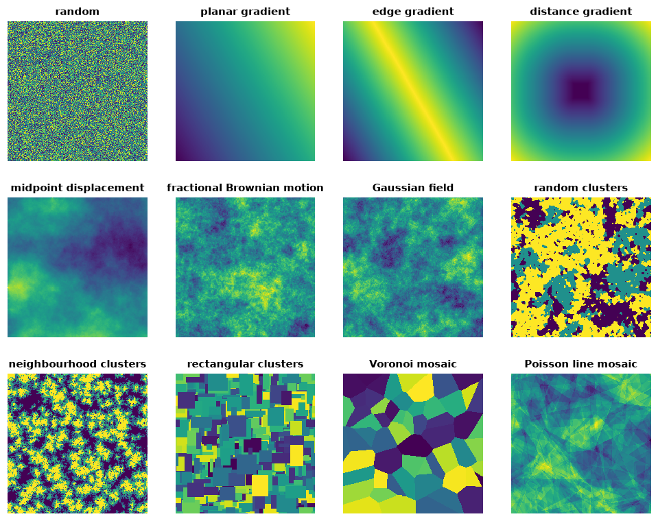
They fall into a few families:

Family	Models	Controls
No structure	random, percolation	habitat share (prob)
Gradients	planar_gradient, edge_gradient, distance_gradient	direction, origin
Fractal surfaces	mpd, fbm	roughness / fract_dim: how quickly detail fades
Random fields	gaussian_field	range of the autocorrelation, nugget
Clusters	random_cluster, neigh, random_rectangular_cluster, curds	compactness and size of the clusters
Mosaics	mosaic_tess, mosaic_gibbs, mosaic_field	number of tiles, spacing of the germs

Continuous models are rescaled to 0-1 by default (rescale=False keeps the raw values). Gradients and random surfaces can be combined with ls.nlm.merge, for instance a regional gradient with local noise:

blend = ls.nlm.merge(models["planar gradient"], models["fractional Brownian motion"], scaling=0.6)

From continuous surfaces to habitat maps

Most analyses need categories. ls.nlm.classify cuts a continuous landscape by class proportions (or by Jenks' natural breaks with n=), and ls.nlm.binarize gives habitat/matrix maps at chosen habitat shares, the highest values becoming habitat:

surface = ls.nlm.fbm(200, 200, fract_dim=1.6, seed=3)
maps = ls.nlm.binarize(surface, [0.2, 0.4, 0.6])     # 1 matrix, 2 habitat
[float((maps.sel(p=b) == 2).mean()) for b in (0.2, 0.4, 0.6)]

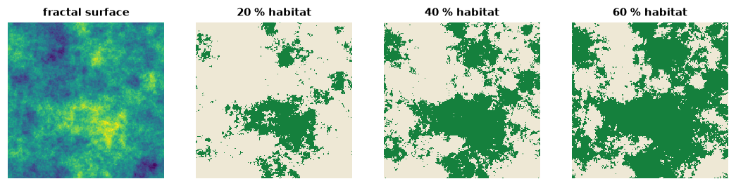
The same surface keeps its structure at every share: the habitat grows from the peaks, and the patches merge as the share rises (the percolation threshold of Learn chapter 3).

A null-model test

Is the forest of the example map more aggregated than chance would make it? We take a corner of the map, measure the aggregation index (ai) of its forest, and compare it with 99 random maps and 99 fractal maps with the same amount of forest:

forest = ls.load_raster(ls.example_data("input")).values[:250, :250]
habitat = np.where(forest == 2, 2, 1)             # the few missing cells as matrix
share = float((habitat == 2).mean())


def aggregation(m):
    table = ls.landscape_metrics(np.asarray(m), level="class", metric="ai")
    return float(table.loc[table["class"] == 2, "value"].iloc[0])


observed = aggregation(habitat)
random_ai = [aggregation(ls.nlm.binarize(ls.nlm.random(250, 250, seed=s), share)) for s in range(1, 100)]
fractal_ai = [aggregation(ls.nlm.binarize(ls.nlm.fbm(250, 250, fract_dim=1.5, seed=s), share)) for s in range(1, 100)]
observed, max(random_ai), min(fractal_ai), max(fractal_ai)

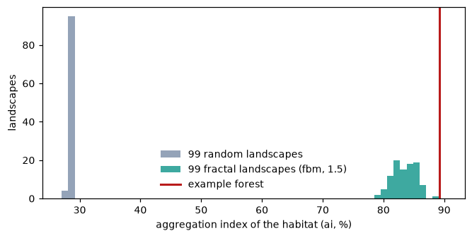
The forest's aggregation index is 89.2 %. Random maps with the same 28 % of forest reach at most 29 %: the pattern is certainly not chance. The sharper question is whether the forest is more aggregated than a spatially autocorrelated surface of that roughness: the 99 fractal landscapes score 79 to 89 %, all of them below the forest. The rank of the observed value among the replicates is the test: above all 99 replicates, the forest is more aggregated than both null models at the 1 % level (one-sided).

The same design works for any response: the output of a dispersal model, an occupancy map, a connectivity index. Use models whose structure matches the hypothesis: random tests for any structure at all, fbm and gaussian_field for aggregation beyond a given autocorrelation, cluster and mosaic models for patch shapes and sizes.

Reproducing NLMR

Every model follows its NLMR counterpart value for value. The seed is NLMR's user_seed:

# R
library(NLMR)
r <- nlm_mpd(ncol = 129, nrow = 129, roughness = 0.7, user_seed = 42)

# Python: the same values
m = ls.nlm.mpd(129, 129, roughness=0.7, seed=42)

A few models behave in NLMR differently from what their documentation says; nlmr_compat=True (the default) keeps these behaviours so that results match, and nlmr_compat=False does what the documentation promises:

Model	NLMR's behaviour (nlmr_compat=True)	nlmr_compat=False
mpd	square output of max(nrow, ncol) ± 1 cells	the size asked for
distance_gradient	origin as rows then columns; great-circle distances in metres for rasters up to 360 × 90 cells	origin as columns then rows; Euclidean distances
mosaic_field	n = 1 sums three mosaics	one mosaic
mosaic_tess, mosaic_gibbs	values given in GEOS's order of the Voronoi cells (with shapely)	each germ its own value

nlm_fbm and nlm_gaussianfield print a message in NLMR 1.4 (RandomFields left CRAN); Landschaft gives the values of the replacements NLMR ships internally (simulate_fbm, simulate_gaussian_field).

Speed

The models run in C++ with OpenMP. The random numbers are drawn in NLMR's order, and everything else runs in parallel: the fast Fourier transforms of the spectral models, the diamond-square steps, the labelling and gap filling of the cluster models, the rasterisation of the mosaics. Typical gains over NLMR are 2 to 8 times for the models NLMR computes in C++ or with FFTs, and 100 to 6000 times for those it computes cell by cell in R (percolation, random_cluster, mosaic_field); see the benchmarks.