Distance & restoration
Where would restoring habitat help the most? How far is every point from the forest, and how costly is it to cross the land in between? This tutorial measures distances and costs, finds the cheapest routes between habitat areas and scores a landscape's restoration potential.
You will learn to:
- map distances to the habitat edge, inside and outside the habitat;
- score how connected a habitat is and how much could be gained;
- turn distance into a resistance to movement;
- compute accumulated cost from a set of cells;
- find the cheapest route between two habitat areas and its cost;
- delimit the zones of influence of large habitat objects.
import numpy as np
import landschaft as ls

forest = ls.load_raster(ls.example_data("input"))   # 0 missing, 1 background, 2 forest
Distance to the habitat edge
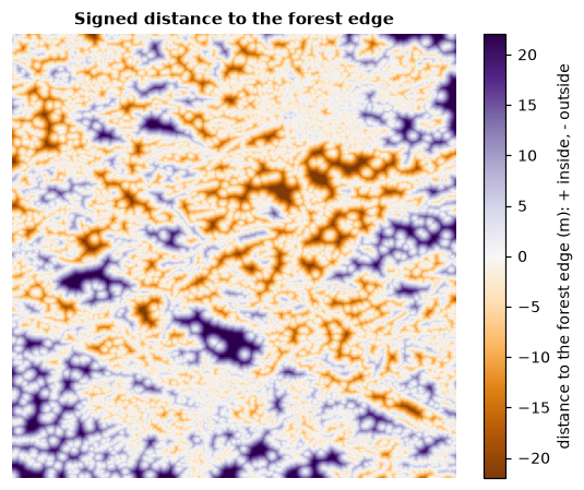
distance.signed_distance holds, for every pixel, the straight-line distance
to the forest edge: positive inside the forest (how deep in the interior),
negative outside (how far from the nearest forest). pixel_size converts
pixels to metres; mean_fg_distance, max_bg_distance and the others
summarise the map.
Restoration status
How connected is the habitat, and how much could it gain from reconnecting its pieces?
status = ls.restoration_status(forest)
status.nr_comp, round(status.doc, 1), round(status.rest_pot, 1)
| Value | Meaning |
|---|---|
nr_comp |
number of separate habitat objects |
eca |
equivalent connected area, pixels: the size of one object with the same connectivity |
doc |
degree of connectivity, eca over the total habitat, % |
rest_pot |
restoration potential, 100 − doc: what reconnecting everything would add |
larg_obj, aps |
largest object and average object size, pixels |
Here about half of the habitat is effectively connected; the rest is the potential gain from restoration.
From distance to resistance
Movement through non-habitat is often harder the further it is from habitat.
distance_to_resistance turns the distance to the forest into a resistance
map: 2 on the forest, from 3 next to it up to 100 far away, 0 on missing data.
Any resistance map with values from 1 to 100 works in the tools below, e.g. one derived from land cover as in the circuit connectivity tutorial.
Cheapest routes between two habitat areas
Mark the two areas to connect. Here we take the two largest forest objects found by accounting:
objects = ls.accounting(forest)
ids = objects.ids.values
first, second = objects.largest[0][0], objects.largest[1][0]

marker = np.zeros(forest.shape, dtype="uint8")
marker[ids == first] = 1           # object A
marker[ids == second] = 2          # object B
marker[forest.values == 0] = 3     # missing: not crossed
The isochrone map accumulates the cost of travelling from A to B through every pixel and draws the cheapest route:
route = ls.isochrone_map_ab(resistance, marker)
ls.plot(route)        # the cost map, the corridor and the path
ls.save(route, "route_ab")
route.min_cost, int(np.asarray(route.lcp).sum())
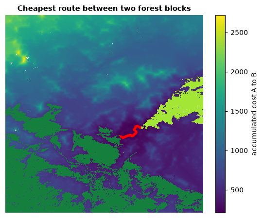
route.cost is the accumulated cost through each pixel (lowest along the
route), route.lcp the path itself and route.map the same in 0–100 display
codes. ls.isochrone_map(resistance, marker) gives the cost outward from A
alone (travel-time rings).
Cost distance and least-cost paths
The same building blocks, separately:
cost = ls.cost_distance(resistance, marker == 1)                 # accumulated cost from A
path = ls.least_cost_path(resistance, marker == 1, marker == 2)
path.path_length, path.rest_pixels, path.expense
path.lcp_mask is the path, path.rest_pixels the number of non-habitat
pixels on it (what would have to be restored) and path.expense its total
cost. ls.restoration_corridor(forest, resistance, marker == 1, marker == 2)
also reports how much the connectivity of the whole landscape would gain if
that corridor were restored, and how efficient the investment is.
Zones of influence
Which large habitat object is the nearest to every point of the matrix?
Objects of at least min_area pixels each get a zone of the background
closest to them; zones.zones maps them and the lines between zones show
where two objects are equally far. ls.proximity measures how close
neighbouring objects are along those lines.
Experimental
Influence zones and proximity follow the original method but do not yet reproduce its distance transform exactly; results can differ in detail from other implementations.
Next steps
- Current flow instead of a single best route: circuit connectivity.
- Change between two dates: change detection.