Restoration priorities

Where should converted land be restored, and how much of each place, to bring back the most biodiversity, carbon and ecological integrity for a given area or budget? This tutorial builds a complete restoration plan for Serra Verde, the example region of the optimized conservation plans, with the restoration problem of ls.prioritize: the model of Strassburg et al. (2020), Global priority areas for ecosystem restoration, solved exactly.

You will learn to:

• find the original vegetation of converted land, and what restoring it brings back;
• measure each species' habitat today and before conversion, and what every restored cell gives it;
• turn habitat into extinction risk, and see why the rarest species drive the plan;
• solve a plan for an area target, and compare it with restoring everywhere alike;
• add ecosystems, carbon and ecological intactness, and weigh them against each other;
• plan with a budget, find the cheapest plan for a benefit, and set targets per region;
• map priorities as a gradient, and plan conservation and land conversion with the same model;
• report the uncertainty of the results, and save them.

Background

Chapter 9 of the course introduces restoration, and chapter 12 conservation planning: targets, costs, objectives and why a plan made by optimization does better than ranking cells one by one.

How the model works

A converted cell is rarely all pasture or all crops: the model works with the share of every land-cover class in each cell, and decides the share of each cell to restore, from 0 to its converted share. Restoring a cell turns its pasture and cropland back into the natural vegetation that was there, which adds habitat to the species that live in that vegetation. The benefit of a plan is the sum of what it brings:

Benefit	What restoring a cell adds	Method
species	less extinction risk for the species whose habitat it grows	add_extinction_risk_benefit
ecosystems	less risk of collapse for its ecoregion	add_extinction_risk_benefit with ecosystem_areas
carbon	the carbon the restored vegetation holds	add_linear_benefit
intactness	less human pressure on it and its surroundings	add_intactness_benefit

The extinction risk of a species follows the species-area relationship: with a share r of its original habitat left, its risk is 1 − r^z (z = 0.25). The curve is steep for species that have lost much habitat and flat for those that have lost little, so the same hectare restored avoids far more risk for a rare species than for a common one. Because the curve is concave, a plan that cannot be improved locally is the best of all, which solve() finds and proves: it returns the plan with a bound on the best possible benefit.

The data

Serra Verde ships with the layers a restoration plan needs: the share of six land-cover classes in every 1 km cell, the natural cover in the past, the human footprint, four ecoregions, the carbon restored vegetation would hold, and the cost of land.

import numpy as np
import landschaft as ls

P = ls.prioritize
cover = ls.load_raster(P.example_data("land_cover"))          # share of each class (6 bands)
past = ls.load_raster(P.example_data("past_cover"))           # natural classes in the past (3 bands)
features = ls.load_raster(P.example_data("features"))         # habitat suitability of 8 features
footprint = ls.load_raster(P.example_data("footprint"))       # human footprint index (0-50)
ecoregions = ls.load_raster(P.example_data("ecoregions"))     # 4 ecoregions
carbon = ls.load_raster(P.example_data("carbon_potential"))   # t/ha in restored vegetation
cost = ls.load_raster(P.example_data("cost"))                 # thousand USD per km²
regions = ls.load_raster(P.example_data("regions"))           # 3 administrative regions

natural = ["forest", "savanna", "mangrove"]
anthropic = ["pasture", "cropland"]
print([str(b) for b in cover.band.values])
print(f"pasture and cropland: {float(cover.sel(band=anthropic).sum()):.0f} km²")

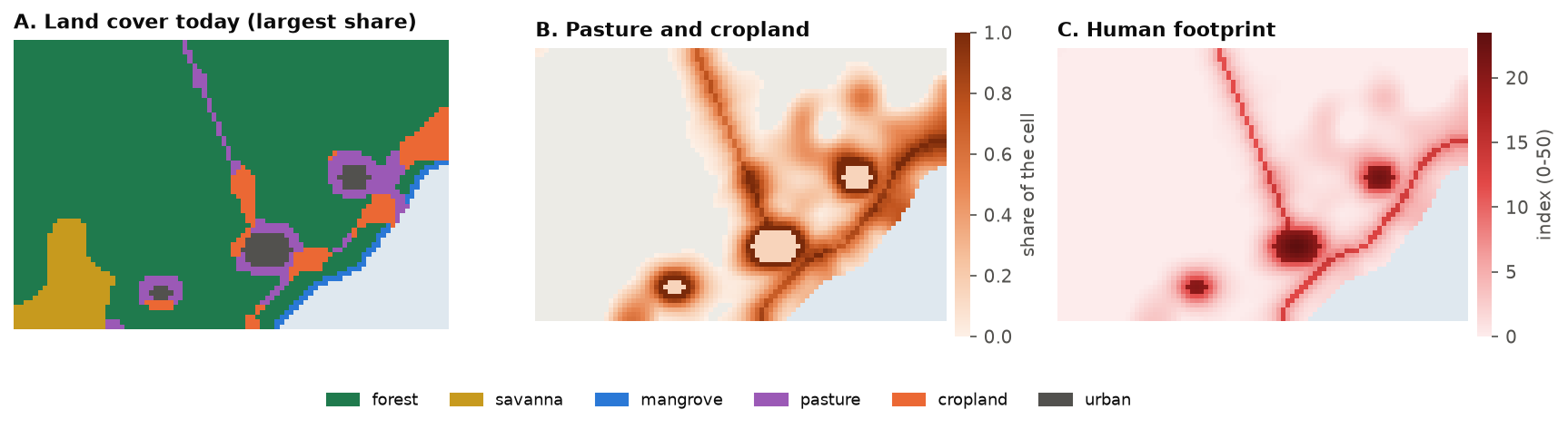
Pasture and cropland cover 916 km², along the roads and around the three cities. The cities themselves (urban) are neither natural nor anthropic here: they are not restored. Your own data can have any classes; the land cover is a (band, y, x) raster whose band names are the classes, the shares of a cell summing to at most 1.

Step 1: the original vegetation

What would grow back on a converted cell? ls.original_vegetation gives the anthropic share of each cell back to the natural classes, in the proportions they had there in the past. Where the past map has no natural cover left, or the cell is almost all converted (above threshold, 95 %), it uses the proportions of the cell's ecoregion. Compute them from the past map, as the mean proportions of its cells:

props = past / past.sum("band")                 # the natural classes' proportions in each cell's past
eco_props = props.copy()
codes = ecoregions.values
for code in np.unique(codes[np.isfinite(codes)]):
    inside = codes == code
    eco_props.values[:, inside] = np.nanmean(props.values[:, inside], axis=1)[:, None]

veg = ls.original_vegetation(cover, natural, anthropic, past=past, ecoregions=eco_props)
print(veg.classes)
source, cells = np.unique(veg.source.values[np.isfinite(veg.source.values)], return_counts=True)
print(dict(zip(source.astype(int).tolist(), cells.tolist())))      # cells per source

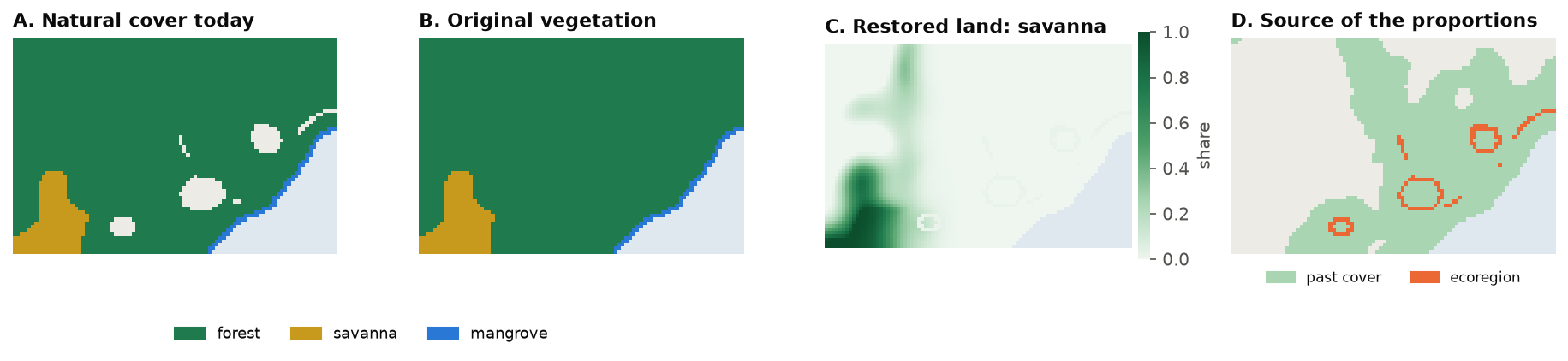
The result holds the original cover (one band per natural class), the proportions restored land becomes in each cell (restore), the source of those proportions (0 the past, 1 the ecoregion, 2 a fallback) and the anthropic share: the land a plan can restore. Here the past map covers almost every cell; the ecoregion fills the 117 nearly converted cells at the edge of the cities (map D).

No past map?

Without past, the current natural shares are used; without ecoregions, equal proportions. Equal proportions put mangrove inland next to the cities, so give the ecoregions whenever a cell can be fully converted. restore_to="current" makes restored land take the cell's current natural classes instead.

Step 2: the habitat of every species

A species' area of habitat is the part of its range covered by the natural classes it lives in. With land-cover shares, every cell of the range counts for its area times the share of those classes. Given the original vegetation, ls.sdm.area_of_habitat also gives the habitat before conversion (the potential) and how much habitat each species gains per unit of each cell restored: what the plan needs.

Here the ranges are the cells where each feature's suitability is above 0; with real data they come from range maps or species distribution models. A table says which classes each species lives in:

ranges = (features > 0).astype("float32")
suitability = {
    "jaguar": ["forest", "savanna"], "lowland_tapir": ["forest"], "harpy_eagle": ["forest"],
    "maned_wolf": ["savanna"], "golden_lion_tamarin": ["forest"],
    "neotropical_otter": ["forest", "mangrove"], "araucaria_forest": ["forest"], "mangrove": ["mangrove"],
}
aoh = ls.sdm.area_of_habitat(ranges, cover, natural, suitability=suitability, original=veg)

t = aoh.table[["species", "current", "potential"]].copy()
t["left"] = t["current"] / t["potential"]
t.round(2)

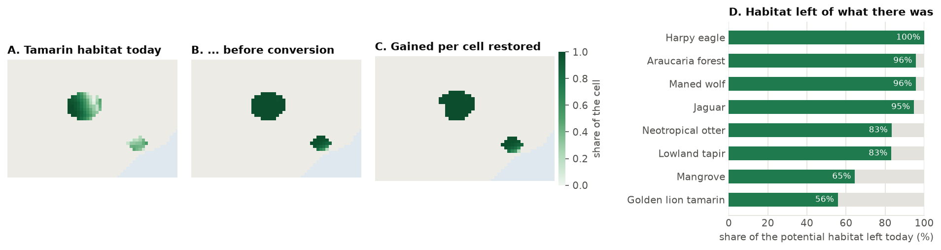
current and potential are in km². The golden lion tamarin keeps 56 % of its habitat and the mangrove 65 %; the harpy eagle, in remote mountain forest, has lost almost none. aoh.gain_map(species) maps the habitat a species gains per cell restored (map C): 1 where a cell would become its habitat in full.

Elevation limits

area_of_habitat(..., elevation=dem, elevation_limits=table) removes from each range the cells outside the species' elevations, as in Brooks et al. (2019).

Step 3: a first plan

A restoration problem starts from the land that can be restored (the original vegetation's anthropic share), adds benefits and targets, and is solved. The first plan restores 100 km², about a ninth of the converted land, for the most extinction risk avoided:

p = (P.restoration_problem(veg)
       .add_extinction_risk_benefit(aoh, name="species")
       .add_area_target(100))                     # km², at most
plan = p.solve()
print(plan.status, f"{plan.area:.1f} km²", f"benefit {plan.benefit:.4f}, bound {plan.bound:.4f}",
      f"{plan.seconds:.2f} s")
print(f"{p.n} cells can be restored; the plan restores {int((plan.values > 0).sum())} of them, "
      f"{int((plan.values >= p.upper - 1e-9).sum())} in full")

plan.restored is the plan as a raster: the share of each cell restored (NaN where nothing can be). The status optimal means the bound and the benefit agree within the tolerance (add_highs_solver(tolerance=...), 1e-7 by default): no plan of 100 km² avoids more risk.

How does each species fare? eval_risk_reduction gives every species' habitat and risk before and after:

rr = P.eval_risk_reduction(p, plan)
rr.table[["species", "risk_before", "risk_after", "reduction"]].round(4)

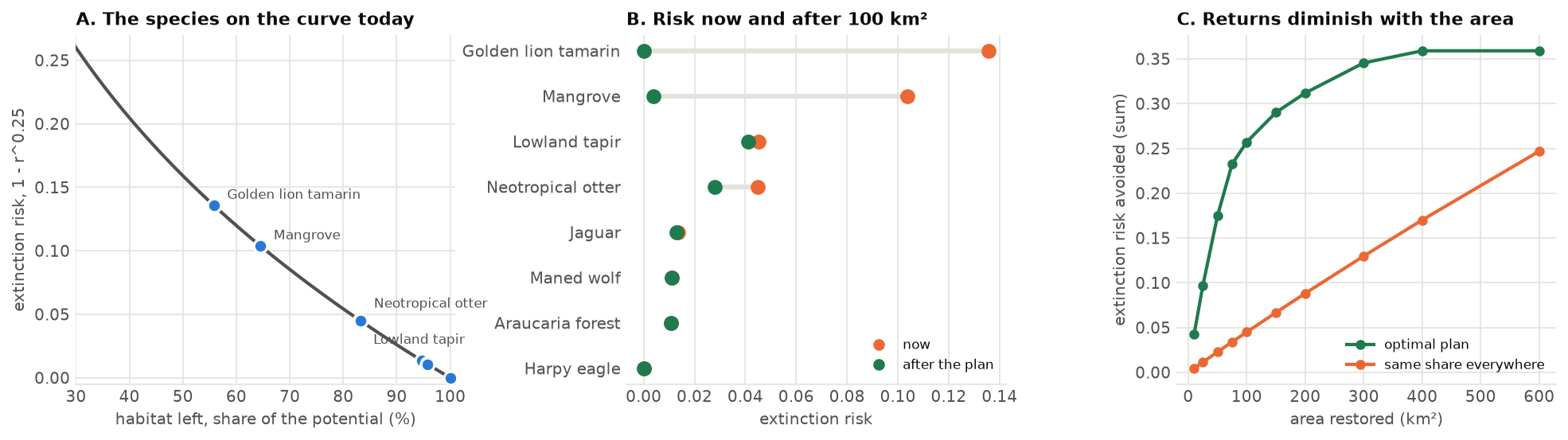
The plan goes almost entirely to the two species furthest down the curve (map A): it restores the golden lion tamarin's forest and the mangrove to (nearly) their potential, which removes nearly all their risk (B), and gives the otter part of what it lost. The widespread species gain little: restoring their habitat would avoid little risk. Past a point, more area buys less and less (C): once the rare species are back to their potential, each km² goes to species with flatter curves.

Compared with restoring everywhere alike

The same 100 km² spread over every converted cell in proportion to its converted share (uniform), and the procedure of the original model (method="steps": cells ranked by benefit, the target met in steps with the benefits recomputed between them):

uni = p.uniform()
steps = p.solve(method="steps", steps=10)
print(f"optimal {plan.benefit:.4f}, steps {steps.benefit:.4f}, same share everywhere {uni.benefit:.4f}")

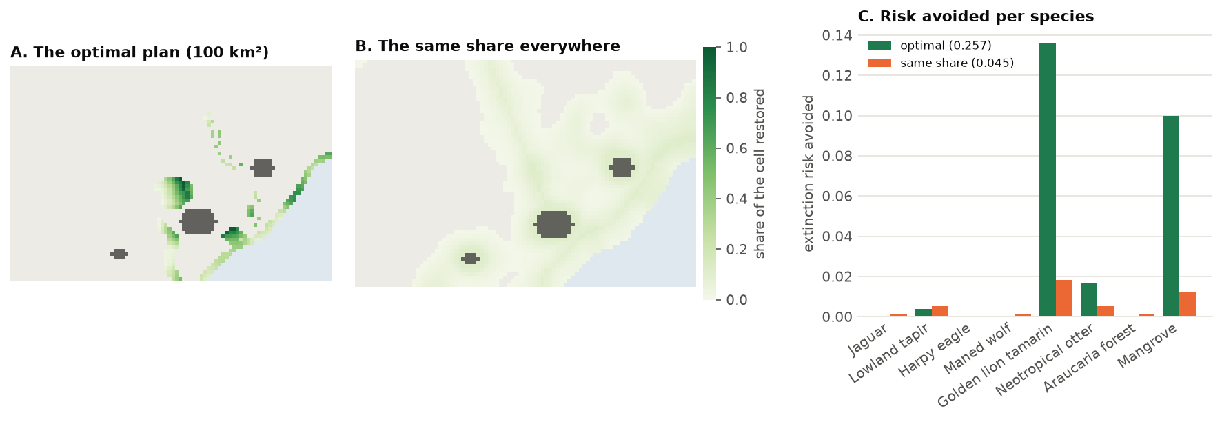
Spreading the effort avoids almost six times less risk (0.045 against 0.257). The stepwise procedure comes close here, but it is a heuristic: it gives no bound, and on other data its result depends on the number of steps.

Step 4: more benefits

Ecosystems

The risk of collapse of an ecosystem follows the same curve, with the natural area of its ecoregion now and before conversion. ecosystem_areas gives them in the form add_extinction_risk_benefit takes:

eco = P.ecosystem_areas(cover, natural, anthropic, ecoregions)
eco.table[["species", "current", "potential"]].round(1)   # "species": the ecoregion's code

The coast (ecoregion 1) and the lowland forest (2) have lost about a third of their area; the montane forest (3) and the savanna (4) little.

Carbon

Carbon is a linear benefit: each km² restored adds its carbon, whatever else is restored. The map is in t/ha; in million tonnes per km² it is carbon * 100 / 1e6:

carbon_mt = carbon * 100 / 1e6                   # Mt of carbon per km² restored

Ecological intactness

The intactness of a cell (Beyer et al. 2020) is high when it and its surroundings bear little human pressure. It comes from the human footprint: a cell's quality is q = exp(−γ HFI), and its intactness the mean of (q_cell q_neighbour)^z over the neighbours within a radius, weighted down with distance. Restoring a share of a cell lowers its footprint by the pressure of the land restored, here 4 for pasture and 7 for cropland (Venter et al. 2016):

reduction = ((4 * cover.sel(band="pasture") + 7 * cover.sel(band="cropland"))
             / cover.sel(band=anthropic).sum("band")).fillna(0)
q = ls.intactness(footprint, radius=3)                       # radius in cells
gain = ls.intactness_gradient(footprint, reduction, radius=3)  # what restoring each cell adds
print(f"mean intactness {float(q.mean()):.3f}")

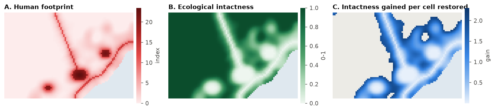
intactness_gradient is the derivative of the total intactness of the landscape with respect to the share of each cell restored: the cell's own intactness rises, and so does that of its neighbours. It is highest at the fringe of the converted land, where restoring one cell reconnects intact surroundings; in the middle of a city's footprint a restored cell stays low in quality and adds little. add_intactness_benefit takes the footprint and the reduction and computes it.

Putting them on one scale

The four benefits are in different units: a risk avoided, a few million tonnes of carbon, a sum of intactness in the hundreds. Weights of 1 would let the largest number win. A simple, transparent choice is to divide each benefit by the most it can reach alone, so each counts from 0 to 1:

base = P.restoration_problem(veg).add_area_target(100)
benefits = {
    "species": lambda q, w=1.0: q.add_extinction_risk_benefit(aoh, weight=w, name="species"),
    "ecosystems": lambda q, w=1.0: q.add_extinction_risk_benefit(eco, weight=w, name="ecosystems"),
    "carbon": lambda q, w=1.0: q.add_linear_benefit(carbon_mt, weight=w, name="carbon"),
    "intactness": lambda q, w=1.0: q.add_intactness_benefit(footprint, reduction, radius=3, weight=w,
                                                            name="intactness"),
}
best = {name: add(base).solve().benefit for name, add in benefits.items()}   # each benefit alone
print({k: round(v, 4) for k, v in best.items()})

multi = base
for name, add in benefits.items():
    multi = add(multi, 1 / best[name])
both = multi.solve()
share = {k: round(v / best[k], 3) for k, v in both.benefits.set_index("benefit")["value"].items()}
print(both.status, share)

The plan with all four reaches 99 % of the best for the ecosystems, 87 % for carbon, 78 % for the species and 65 % for intactness: each gives up a little, none is sacrificed.

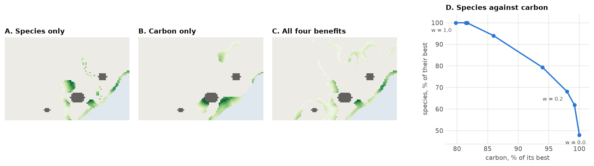
Each benefit alone asks for different places (maps A and B): the species need the tamarin's forest and the mangrove; carbon, the wet lowlands by the coast. To see the trade-off, change the weight w between two benefits and trace the curve (D):

for w in (0.0, 0.2, 0.5, 1.0):
    q = benefits["carbon"](benefits["species"](base, w / best["species"]), (1 - w) / best["carbon"])
    v = q.solve().benefits.set_index("benefit")["value"]
    print(f"w = {w:.1f}: species {v['species'] / best['species']:.0%}, carbon {v['carbon'] / best['carbon']:.0%}")

The curve bends: carbon alone (w = 0) gets the species 48 % of their best; w = 0.2 gets them 68 % for 2 % less carbon, and w = 0.5 their best for 82 % of the carbon. Planners pick a point on it with the people involved; the weights are a choice, not a fact of the data.

Step 5: costs and budgets

Restoring costs money: the land, the work, the income the land no longer gives. add_budget limits the spending; the cost is per km² restored:

for budget in (2000, 5000, 8000):                 # thousand USD
    s = p.add_budget(budget, cost).solve()
    print(f"{budget / 1000:.0f} million USD: {s.area:5.1f} km², benefit {s.benefit:.4f} ({s.status})")

The inverse question, how cheaply can a benefit be reached, is add_min_cost_objective. The cheapest plan for 95 % of the first plan's benefit:

plan_cost = float(np.nansum(plan.restored.values * cost.values))
cheap = p.add_min_cost_objective(0.95 * plan.benefit, cost).solve()
print(f"first plan {plan_cost / 1000:.2f} million USD; for 95 % of its benefit {cheap.cost / 1000:.2f} million "
      f"USD and {cheap.area:.0f} km² ({cheap.status})")

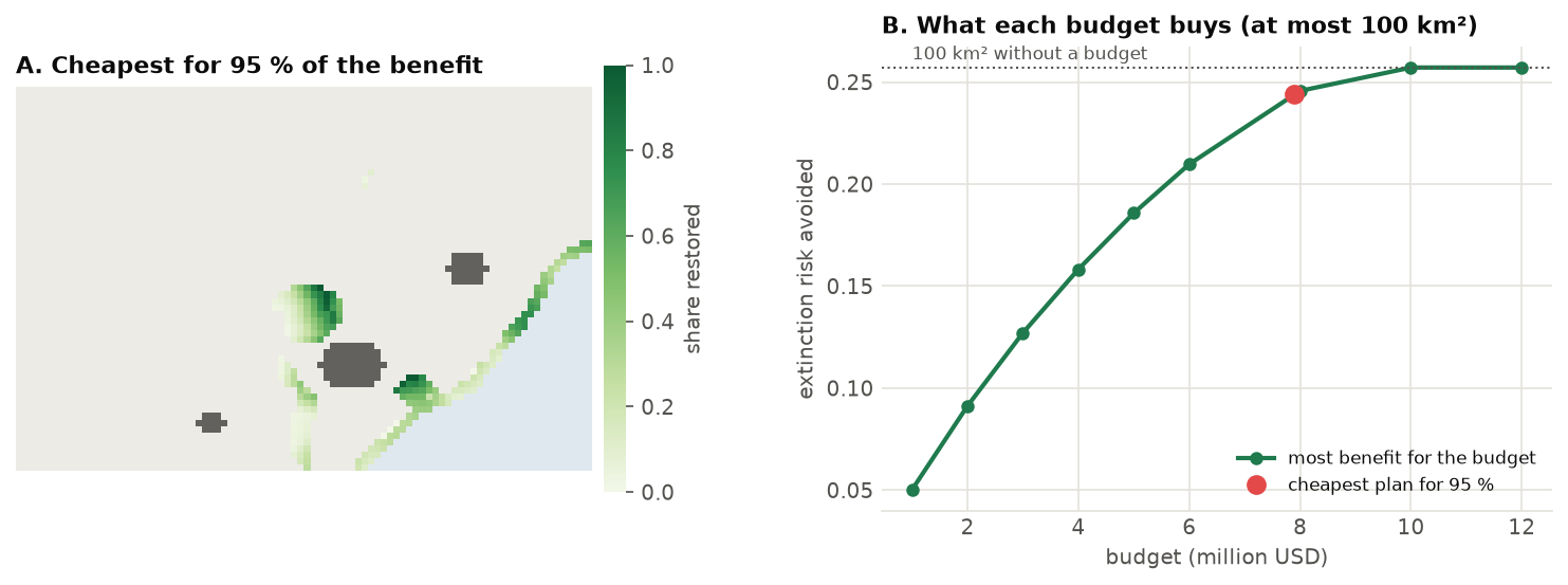
The last 5 % of the benefit costs 1.3 million USD, 15 % of the first plan's cost. Past about 10 million USD the area target, not the budget, limits the plan (B).

Evaluate any plan

p.evaluate(restored) computes the benefits, area and cost of any plan, a raster of shares restored: a plan drawn by hand, from another tool or from a previous year.

Step 6: targets per region

Plans often have to share the effort: every municipality, state or watershed restores its part. add_area_target takes a raster of regions and a target for each (a mapping, or a table with the columns region, target and optionally sense):

by_region = (P.restoration_problem(veg)
               .add_extinction_risk_benefit(aoh, name="species")
               .add_area_target({1: 30, 2: 40, 3: 30}, regions=regions))
shared = by_region.solve()
for r in (1, 2, 3):
    inside = regions.values == r
    print(f"region {r}: {np.nansum(np.where(inside, plan.restored.values, 0)):5.1f} km² without regional "
          f"targets, {np.nansum(np.where(inside, shared.restored.values, 0)):5.1f} km² with them")
print(f"benefit {shared.benefit:.4f} against {plan.benefit:.4f}")

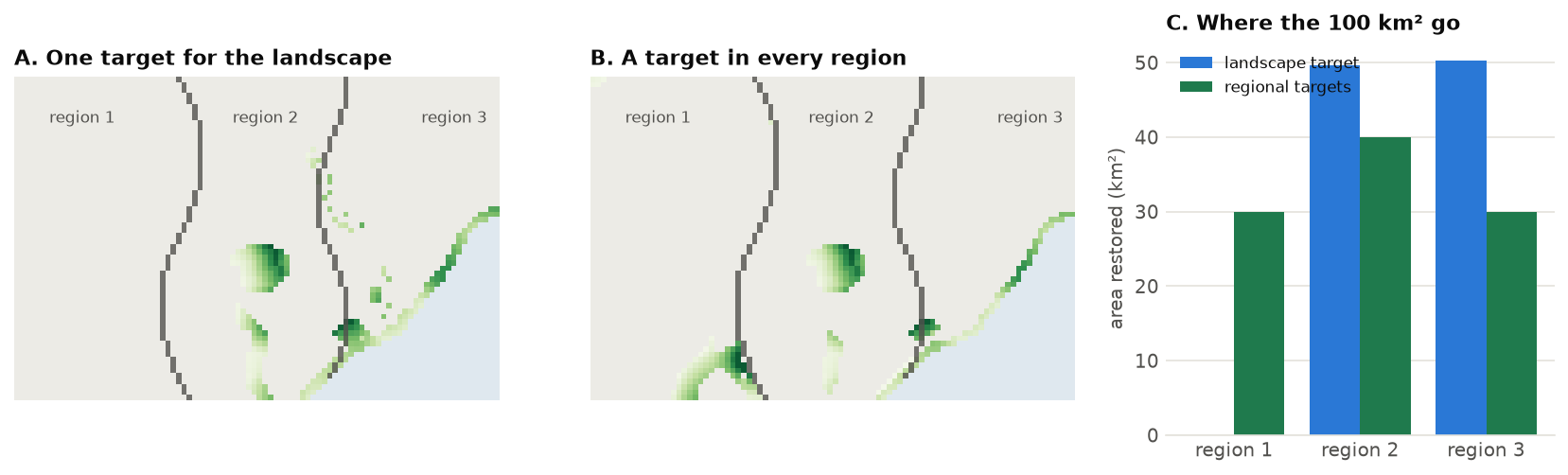
Without regional targets, region 1 gets nothing: its species are in good shape. Sharing the effort costs 9 % of the benefit (0.234 against 0.257), the price of the rule, which a planner can now put in front of decision makers. Use sense=">=" for minimum targets (each region restores at least its part) and "=" for exact ones.

Step 7: a priority gradient

A plan for 100 km² does not say where to start. tradeoff solves the plans of a growing target, each containing the previous one (nested=True, the default), and maps how early every cell enters: a priority gradient.

curve = p.tradeoff([0.25, 0.5, 0.75, 1.0])     # 25, 50, 75 and 100 km²
print(curve.table[["level", "area", "benefit", "status"]].round(4))
g = curve.gradient.values                      # 4: in the first 25 km², 1: only in the last
print({int(k): int(n) for k, n in zip(*np.unique(g[np.isfinite(g)], return_counts=True))})

The first quarter of the area avoids 38 % of the risk the whole plan avoids (0.097 of 0.257), the first half 68 %: the gradient is steep, and the 67 cells of level 4 are where to begin. Each level is the best plan that contains the previous ones; nested=False solves every level on its own (the trade-off frontier, plans that need not contain each other). Here both agree to the fourth decimal: the best 50 km² contain the best 25 km². method="steps" gives the original model's gradient for comparison.

Step 8: conserving and converting

The same model answers two more questions. Which natural land to keep? With conservable= the units are the natural land, and the baseline loses what is threatened (threat, the share lost without protection: here more where the human footprint is high); conserving keeps it. Where to meet a demand for land? With convertible= the plan converts natural land where it costs the least benefit, and with restorable too it can restore elsewhere what it converts. Both need the habitat each species loses per unit of natural land, loss=True:

aoh = ls.sdm.area_of_habitat(ranges, cover, natural, suitability=suitability, original=veg, loss=True)
nat = cover.sel(band=natural).sum("band")           # the natural share of every cell
keep = (P.restoration_problem(conservable=nat, threat=(footprint / 20).clip(0, 1))
          .add_extinction_risk_benefit(aoh, name="species")
          .add_area_target(100))
kept = keep.solve()
print(kept.status, f"benefit {kept.benefit:.4f}")
P.eval_risk_reduction(keep, kept).table[["species", "current", "baseline", "risk_after"]].round(3)

The baseline is each species' habitat if the threatened land were lost; conserving the best 100 km² avoids a risk of 0.046, mostly for the golden lion tamarin and the mangrove, whose remnants are the most threatened.

swap = (P.restoration_problem(veg, convertible=nat)
          .add_extinction_risk_benefit(aoh, name="species")
          .add_area_target(50, sense="=", action="convert")   # a demand of 50 km² of farmland
          .add_area_target(0, sense="="))                     # no net loss: restore what is converted
both = swap.solve()
print(both.status, {k: round(v, 1) for k, v in both.areas.items()}, f"benefit {both.benefit:.4f}")

The 50 km² are converted outside every species' range, so the plan loses nothing and restores 50 km² where they count most: the same benefit as restoring 50 km² alone (0.175). Converting the same area uniformly would raise the risk by 0.025. The solution has a converted map beside restored.

Projections of land demand per region (from an economic model, say) go in with add_projected_change: a region that spares land restores it, one that needs land converts it, each its projected change:

proj = (P.restoration_problem(veg, convertible=nat)
          .add_extinction_risk_benefit(aoh, name="species")
          .add_projected_change({1: -30, 2: 20, 3: 40}, regions))    # km²: region 1 needs 30
s = proj.solve()
for r in (1, 2, 3):
    inside = regions.values == r
    print(f"region {r}: restores {np.nansum(np.where(inside, s.restored.values, 0)):.0f} km², "
          f"converts {np.nansum(np.where(inside, s.converted.values, 0)):.0f} km²")

A plan that only restores cannot convert: there the land demanded is taken from the restoration (compensate=True), regions 2 and 3 restoring 10 and 20 km² of the 30 km² spared on balance. ecosystem_targets shares a target among ecoregions for the least risk of collapse, a table of targets per region for add_area_target.

Step 9: uncertainty

The exponent z of the species-area relationship is uncertain: 0.25 is a typical value, but estimates vary from about 0.15 to 0.35 (the original model uses a standard deviation of 0.1). eval_risk_reduction(z_sd=...) propagates it to the total by the delta method; ls.uncertainty.interval turns it into a confidence interval:

ru = P.eval_risk_reduction(p, plan, z_sd=0.1)
low, high = ls.uncertainty.interval(ru.total, ru.sd)
print(f"risk avoided {ru.total:.3f} ± {ru.sd:.3f} (95 %: {low:.3f} to {high:.3f})")

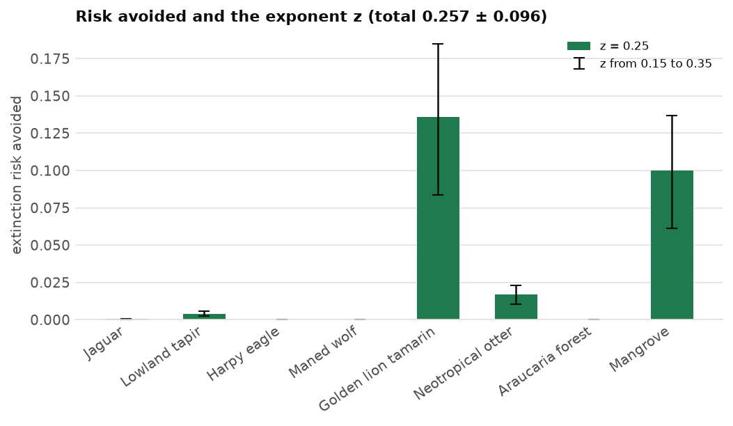
The species' z err together (method="correlated", the default) when they come from one study; "independent" treats them as separate estimates and gives a smaller deviation. The z of each species can also be set: add_extinction_risk_benefit(aoh, z={"golden_lion_tamarin": 0.3}).

The same holds for any linear total. With an error of 25 % in each cell's carbon, ls.uncertainty.sum_sd gives the deviation of the plan's carbon, independent errors or fully correlated (a bias of the carbon map):

on_plan = np.nan_to_num(plan.restored.values)               # km² restored per cell (cells of 1 km²)
total = float(np.nansum(carbon.values * 100 * on_plan))     # tonnes
sd = 0.25 * carbon.values * 100
print(f"carbon {total / 1e6:.3f} Mt; sd {ls.uncertainty.sum_sd(sd, weights=on_plan) / 1e6:.3f} Mt if independent, "
      f"{ls.uncertainty.sum_sd(sd, weights=on_plan, correlation=1.0) / 1e6:.3f} Mt if correlated")

ls.uncertainty also has product_sd, delta_method and monte_carlo for other combinations (API).

Saving and sharing

Every result saves in one call. A plan becomes a folder with the shares restored (restored.tif), the benefits (benefits.csv) and a summary (summary.json); a single map is one GeoTIFF:

plan.save("restoration_plan")                          # restored.tif, benefits.csv, summary.json
rr.save("risk_by_species")                             # the table per species and the totals
veg.save("original_vegetation")                        # original.tif, restore.tif, source.tif, anthropic.tif
ls.write_raster(plan.restored, "restored_share.tif")   # just the map
page = ls.plot(plan.restored, show=False)              # an interactive map

Going further

• Partial benefits. add_extinction_risk_benefit(aoh, restoration_discount=0.3) counts restored land as 70 % habitat, for young or degraded restoration; it can differ per species.
• Limits per cell. restoration_problem(veg, limit=0.5) restores at most half of each cell's converted land; limit can be a raster (0 on land that must stay in production).
• Sense of the area target. add_area_target(100, sense="=") restores exactly 100 km²; ">=" with a budget asks for at least that area.
• Larger landscapes. The exact method scales with the cells: its linear programs have only the problem's rows (targets and budget), and with a single area target or budget none is needed. 9 x 10⁶ cells and 5000 species solve, proven, in about 10 s.
• Exact intactness. add_intactness_benefit(..., form="exact") optimises the total intactness itself, not its slope at the start: it pays where the footprint can be cleared. The total intactness is not concave, so the plan is a local optimum with a bound on the best (status "local" unless they meet).
• Restoration in other planners. To choose whole cells against targets, use optimized conservation plans with the gains as features (recipe); to restore corridors between habitat patches, see distance and restoration.
• The API reference lists every method; original vegetation and intactness and area of habitat are general tools.

References

• Beyer, H. L., Venter, O., Grantham, H. S. & Watson, J. E. M. (2020). Substantial losses in ecoregion intactness highlight urgency of globally coordinated action. Conservation Letters 13, e12692.
• Brooks, T. M. et al. (2019). Measuring terrestrial area of habitat (AOH) and its utility for the IUCN Red List. Trends in Ecology & Evolution 34, 977-986.
• Strassburg, B. B. N. et al. (2020). Global priority areas for ecosystem restoration. Nature 586, 724-729.
• Venter, O. et al. (2016). Sixteen years of change in the global terrestrial human footprint. Nature Communications 7, 12558.