Chapter 12.4

Optimization¶

The objective is the question you ask. Two planners with the same data but different objectives get different maps, and both can be right. This chapter shows how to choose the question, how targets and budgets change the answer, and what happens inside the solver that finds it, without needing the mathematics.

In this chapter

the two ways to frame a question: targets or a budget;
the minimum-set problem and the price of targets;
the budget objectives (utility, shortfall, features, extinction risk) and how to choose one;
what a solver does, what an optimality gap means, and how to read a solution;
exact methods against heuristics such as simulated annealing;
the equations, for those who want them.

Two ways to frame the question¶

Almost every conservation question belongs to one of two families.

I know what I need (targets)I know what I have (a budget)

"We must protect 30 % of every ecosystem. What is the cheapest way?"

You fix the targets, and the solver minimizes the cost. This is the minimum-set problem, the classic question of systematic conservation planning.

p.add_min_set_objective().add_relative_targets(0.3)

"We have 20 million dollars. What is the best we can do with it?"

You fix the budget, and the solver maximizes the benefit. There are several ways to define benefit, which is why there are several budget objectives.

p.add_max_utility_objective(20_000)        # costs in thousand USD

The minimum set¶

The minimum-set objective finds the cheapest set of planning units that meets every target. It is the right choice when targets are not negotiable: when they come from law or from an international commitment.

The price of this certainty is that you do not control the cost. It is whatever the targets require:

import numpy as np
import landschaft as ls

P = ls.prioritize
cost = ls.load_raster(P.example_data("cost"))
features = ls.load_raster(P.example_data("features"))
base = P.problem(cost, features).add_min_set_objective().add_binary_decisions()

for t in (0.1, 0.3, 0.5):
    s = base.add_relative_targets(t).solve()
    print(f"{t:.0%} of every feature: {int(s.values.sum())} cells, {s.cost / 1000:.1f} million USD")

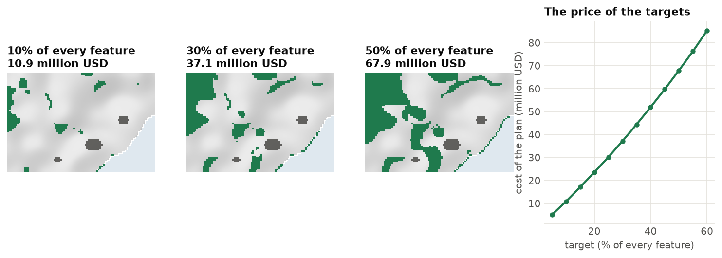
Plans for 10 %, 30 % and 50 % targets, and their cost — Minimum-set plans for Serra Verde with targets of 10 %, 30 % and 50 % of every feature. The cost rises faster than the target: 10.9, 37.1 and 67.9 million USD. Tripling the target from 10 % to 30 % more than triples the cost, because the cheapest places are used first and every further step must buy dearer land.

If the targets cannot be met (say, 60 % of a species whose habitat is half inside cities that were locked out), the problem has no solution, and the solve reports status == "infeasible". Check the feature totals and the locked-out units before raising targets.

Budget objectives¶

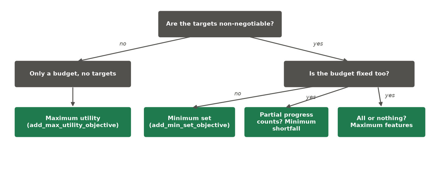
When the money is fixed, you must say what "doing the most" means. ls.prioritize offers the objectives of prioritizr (Hanson et al. 2025) and one of its own:

Objective	What it optimizes within the budget	Good for
`add_max_utility_objective`	the total amount of all features held (weighted)	the most biodiversity per dollar overall; no targets
`add_min_shortfall_objective`	the sum of the shortfalls, each as a share of its target	progress on every feature at once
`add_min_largest_shortfall_objective`	the largest shortfall of any single feature	leaving no feature far behind
`add_max_features_objective`	the number of targets fully met (weighted)	securing as many features as possible completely ("triage")
`add_max_cover_objective`	the number of features held at all, any amount above zero	a first presence of every feature; no targets
`add_max_phylo_div_objective`	the evolutionary history (branch length of a phylogeny) with targets met	the tree of life, not just species counts (Faith 1992)
`add_max_phylo_end_objective`	the same, weighting branches by how restricted they are	phylogenetic endemism (Rosauer et al. 2009)
`add_min_extinction_risk_objective`	the expected loss of species from the species-area relationship	persistence without arbitrary targets

Here are three of them spending the same budget, half of what the 30 % minimum set costs:

budget = 0.5 * base.add_relative_targets(0.3).solve().cost
with_targets = P.problem(cost, features).add_relative_targets(0.3).add_binary_decisions()
plans = {
    "max utility": P.problem(cost, features).add_max_utility_objective(budget).add_binary_decisions(),
    "min shortfall": with_targets.add_min_shortfall_objective(budget),
    "max features": with_targets.add_max_features_objective(budget),
}
for name, q in plans.items():
    s = q.add_highs_solver(gap=0.005).solve()
    held = P.eval_feature_representation_summary(base.add_relative_targets(0.3), s)["relative_held"]
    print(f"{name:13s} targets met: {int((held >= 0.3 - 1e-6).sum())} of 8;  held: {held.round(2).tolist()}")

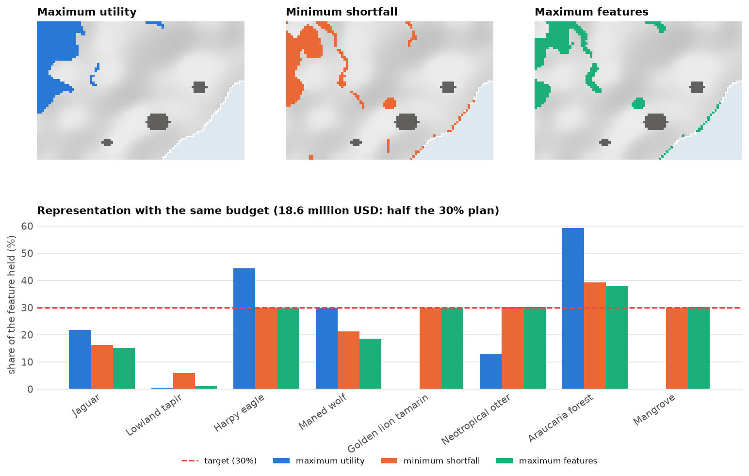
Three objectives spending the same budget — Maximum utility piles up the most total habitat, but in the cheap mountains: it leaves the tamarin and the mangrove with nothing and the tapir with almost nothing. Minimum shortfall and maximum features use the targets to spread the money. They secure the rare features (tamarin, otter, mangrove), the harpy eagle and the araucaria forest, five targets of eight, and share what is left among the widespread ones.

A few lessons from this comparison:

Maximum utility favours widespread, cheap features. Without weights, a km² of common habitat counts as much as a km² of a rare one. Feature weights (add_feature_weights) correct this, or the totals of every feature can be scaled to one before solving.
Minimum shortfall measures gaps as shares of each target, so a small gap for a rare species counts as much as a large gap for a common one. With targets, it is a balanced default.
Maximum features is all or nothing for each feature. It suits cases where partial protection has little value (a population 80 % protected may still collapse), but it abandons the features it cannot fully secure.

Choosing an objective¶

A decision tree for the objective. When not sure, do not pick one budget: draw the whole curve between money and targets (a Pareto front, chapter 12.6). It is often the most useful figure for decision makers.

Extinction risk instead of targets¶

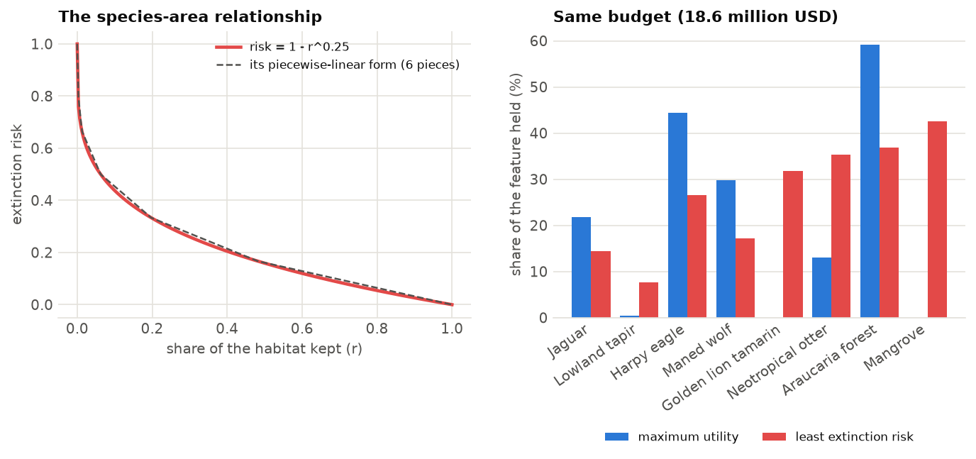
Targets are thresholds: 29 % of a species' habitat counts for nothing if the target is 30 %. Ecology suggests something smoother. By the species-area relationship, the share of species, or of a population's persistence, that a habitat keeps grows as a power of its area, S ∝ A^z with z near 0.25 (Pereira & Daily 2006). The risk of losing a feature when a share r of its habitat is kept is then 1 − r^z. The first losses cost little; the last ones cost much.

add_min_extinction_risk_objective(budget, z=0.25) minimizes the sum of these risks over the features. The curve enters the model as a few straight segments, which keeps it exact at their ends and fast to solve.

risk = P.problem(cost, features).add_min_extinction_risk_objective(budget).add_binary_decisions()
s = risk.add_highs_solver(gap=0.005).solve()
P.eval_extinction_risk(base.add_relative_targets(0.3), s).round(3).tail(3)

The species-area curve and its effect — Left: the extinction risk 1 − r^0.25 as the share r of habitat kept grows, and its piecewise-linear form. The steep start means losing the last fragments of a species is very costly. Right: with the same budget, minimizing risk spreads the habitat across all eight features, while maximum utility concentrates it on a few. The expected number of features lost, the sum of the risks, falls from 4.0 to 2.4.

Inside the solver¶

A problem too large to try every answer¶

Serra Verde has 4825 planning units. Each can be in or out of the plan, so there are 2⁴⁸²⁵ possible plans, a number with 1453 digits. Trying them all is impossible, even on every computer on Earth for the age of the universe. Yet the solve above takes a fraction of a second. How?

ls.prioritize writes the problem as a mixed integer linear program (MILP):

one variable per planning unit, x_i = 1 if it is selected and 0 if not;
an objective: the total cost Σ c_i x_i, to minimize;
constraints: for every feature j, the amount held Σ r_ij x_i must reach its target T_j.

model = base.add_relative_targets(0.3).compile()
model                               # rows: one per target; columns: one per planning unit

A solver is a program, built over decades for airline schedules and supply chains, that searches such models cleverly. ls.prioritize translates the conservation problem into the solver's language and the answer back into maps; you never deal with the solver directly.

In plain words

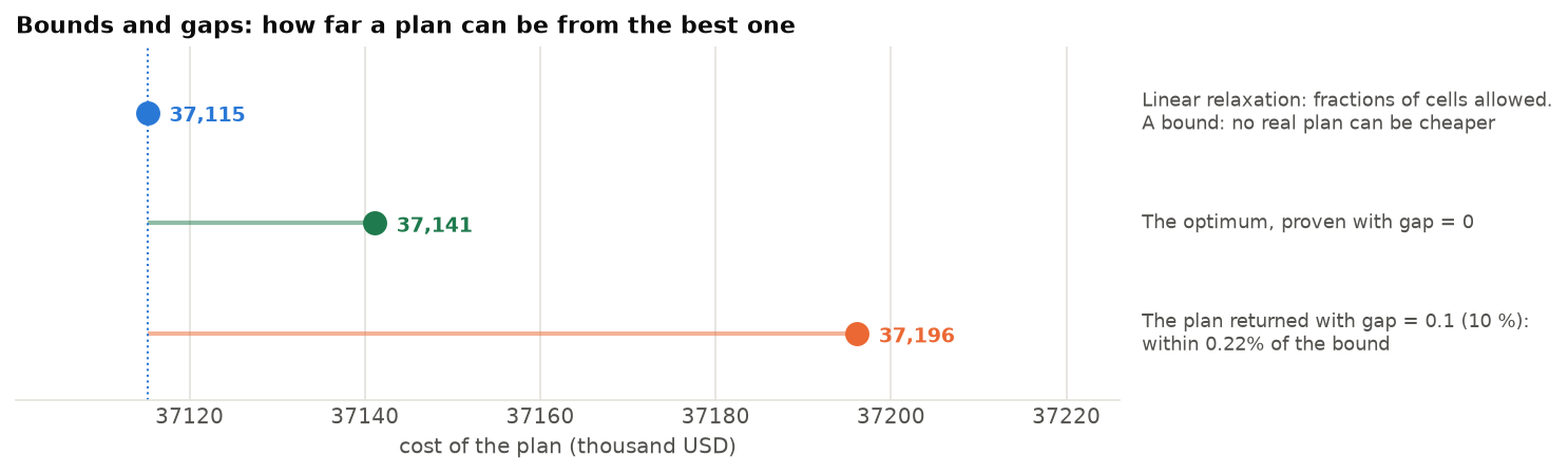
Imagine first allowing fractions of cells: 0.3 of this one, 0.7 of that one. This relaxed problem is easy to solve exactly, and its cost is a bound: no real plan can be cheaper. Then the solver branches. It picks a cell with a fraction and tries two sub-problems, one with that cell fully in and one with it fully out. Any branch whose bound is already worse than the best plan found so far is discarded, along with the billions of plans beneath it. This is branch and bound.

The optimality gap¶

At any moment the solver knows two numbers: the cost of the best plan found and a bound that no plan can beat. Their relative difference is the optimality gap. A gap of 0.01 is a proof: this plan costs at most 1 % more than the best possible one. When the gap reaches the value you asked for, the solver stops.

exact = base.add_relative_targets(0.3).add_highs_solver(gap=0.001).solve()
loose = base.add_relative_targets(0.3).add_highs_solver(gap=0.1).solve()
print(f"gap 0.1%: cost {exact.cost:,.0f}  bound {exact.bound:,.0f}  gap {exact.gap:.3%}")
print(f"gap 10%:  cost {loose.cost:,.0f}  bound {loose.bound:,.0f}  gap {loose.gap:.2%}")

Asked for 0.1 %, the solver returns a plan within 0.01 % of the bound in under a second. Closing the gap completely (gap=0) proves that the optimum is 37,141, but takes about 40 seconds: the last fraction of a percent is usually the slowest part of the proof, and rarely worth it.

Bounds and gaps — The linear relaxation (fractions of cells allowed) gives a bound below every real plan. The optimum lies between it and any plan found. A plan solved to a 10 % gap carries its own proven bound: the optimum cannot be below it. In practice the plans found are often much closer to the optimum than the gap guarantees.

The default gap is 10 %, as in prioritizr: generous, but the plan found is usually much closer (the first plan of this chapter came within 0.2 %). For exploration, 1 to 5 % is plenty and much faster on hard problems; for a final plan, ask for a small gap with add_highs_solver(gap=...) and report it. The status of a solution says how the solve ended: "optimal" (the gap asked for was reached), "time_limit", "infeasible".

Solvers in `ls.prioritize`¶

Solver	Method	When
`add_highs_solver` (default)	exact (MILP), open source, built in	almost always
`add_gurobi_solver`	exact (MILP), commercial, needs a licence	very large or hard models, if you have it
`add_anneal_solver`	simulated annealing, as in Marxan	Marxan comparisons; penalties on huge maps

Behind HiGHS, Landschaft adds engines of its own for the problems that general solvers find hard: covering problems with millions of units, boundary and connectivity penalties, multi-action plans. They start the solver from a near-optimal plan and fix the units whose choice is already proven, so the same models solve in seconds instead of hours. You do not choose them: they run when they apply, and the gap and status keep their meaning.

Exact methods and heuristics¶

There are two families of methods for finding good sets of areas:

	Heuristics (simulated annealing, greedy)	Exact optimization (MILP)
How it works	starts from a random or partial plan and improves it step by step	formulates the problem mathematically and solves it with branch and bound
Quality	no guarantee: the answer can be far from the best, and you cannot tell how far	a proven gap: "at most 1 % dearer than the best possible plan"
Repeatability	different runs give different answers	the same input gives the same answer
Speed	fast, even on huge problems	very fast on most problems; some spatial rules are slow

Marxan (Ball et al. 2009) made simulated annealing the standard tool of conservation planning for two decades. It swaps units in and out at random, accepting worse plans early on (like a metal cooling slowly) to escape poor local solutions. It works well, but it cannot say how good its answer is. Beyer et al. (2016) showed that integer programming finds better plans, often much faster, on the same problems.

anneal = base.add_relative_targets(0.3).add_anneal_solver(num_reps=10, seed=1).solve()
print(f"annealing: {anneal.cost:,.0f}   optimum: {exact.cost:,.0f}   "
      f"({anneal.cost / exact.cost - 1:.1%} dearer)")

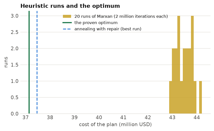
Heuristic runs and the optimum — Twenty runs of Marxan's simulated annealing (2 million iterations each) on the 30 % problem of Serra Verde. They cost from 42.9 to 44.2 million USD, 15 to 19 % more than the proven optimum of 37.1 million, and five of them miss a target. None of them knows how far it is from the best plan. The annealing solver of `ls.prioritize` repairs and trims every run, which brings its best run to 37.5 million, within 1 % of the optimum, and reports the gap to the bound.

Heuristics still have a place: for problems too large or too non-linear for an exact solver, to reproduce a Marxan analysis, and as a starting point (solve(start=...)) for an exact solver.

Weights, locks and other rules¶

The objective and the targets are the core of the question. Real plans add more:

feature weights (add_feature_weights): how much a feature matters in a budget objective, for instance more for threatened or endemic species;
locked units: add_locked_in_constraints (existing reserves, always selected) and add_locked_out_constraints (cities, mines, never selected);
linear constraints (add_linear_constraints): any other limit on a sum over the selected units, such as "at most 2000 km² of farmland" or "at least 500 km² in the north";
penalties (boundary, connectivity, linear): soft preferences that add a cost to undesirable plans, traded off against the objective;
spatial constraints (neighbours, contiguity, corridors): hard rules about the shape of the plan.

Constraints are hard: the plan must obey them. Penalties are soft: the plan pays for breaking them. The next chapter is about the most important of both, the shape of the plan.

protected = ls.load_raster(P.example_data("protected"))
urban = ls.load_raster(P.example_data("urban"))
plan = (base.add_relative_targets(0.3)
            .add_locked_in_constraints(protected)
            .add_locked_out_constraints(urban)
            .solve())
print(f"with reserves and cities: {plan.cost / 1000:.1f} million USD")

The equations¶

You do not need them to use ls.prioritize, but they make precise what each objective means. With x_i ∈ {0, 1} the decision for planning unit i (or 0 ≤ x_i ≤ 1 with proportion decisions), c_i its cost, r_ij the amount of feature j in it, T_j the target of feature j, B the budget and w_j the feature weights:

Objective	Model
minimum set	minimize Σ_i c_i x_i subject to Σ_i r_ij x_i ≥ T_j for every j
maximum utility	maximize Σ_j w_j Σ_i r_ij x_i subject to Σ_i c_i x_i ≤ B
minimum shortfall	minimize Σ_j w_j y_j / T_j subject to Σ_i r_ij x_i + y_j ≥ T_j, y_j ≥ 0, budget
minimum largest shortfall	minimize z subject to z ≥ y_j / T_j for every j, the shortfall rows and the budget
maximum features	maximize Σ_j w_j m_j subject to Σ_i r_ij x_i ≥ m_j T_j, m_j ∈ {0, 1}, budget
minimum extinction risk	minimize Σ_j w_j (1 − v_j) subject to v_j ≤ a_k + b_k (Σ_i r_ij x_i / R_j) for every segment k of r^z, budget

Penalties add terms to the objective. The boundary penalty, for instance, adds p Σ_i,k b_ik (x_i + x_k − 2 x_i x_k) / 2 plus the exposed edges of selected units: the length of the plan's outline, weighted by p (chapter 12.5). The product x_i x_k is written with an extra variable and three linear constraints, which keeps the model linear. Problem.compile() returns the exact model, and it is the same, row by row, as prioritizr's.

Key points

With firm targets, minimize cost (minimum set); with a firm budget, choose what "the most" means.
The cost of a plan grows faster than its targets: the cheapest land goes first.
Maximum utility favours common features; shortfall objectives and weights balance them.
A solver proves how good its plan is: the optimality gap. Heuristics cannot.
Constraints are hard rules; penalties are soft preferences paid for in the objective.

Check your understanding¶

A ministry must protect 30 % of every ecosystem by law and wants to know the cost. Which objective? And an NGO with 5 million dollars?
A plan has a gap of 2 % and costs 40 million. What is the least the best possible plan could cost?
With maximum utility and no weights, why does the plan avoid the mangrove even though it is rare?
Why can't simulated annealing report a gap?

Answers

The ministry: minimum set (targets fixed, cost unknown). The NGO: a budget objective, for instance minimum shortfall if it has targets, maximum utility if not.
About 40 / 1.02 = 39.2 million: the bound proves no plan is cheaper.
Maximum utility adds up amounts. The mangrove's total amount is small, and it grows on dear coastal land, so each dollar buys more total habitat in the cheap mountains. Weights or targets fix this.
A gap needs a bound, a proof that no plan is better. Annealing only compares the plans it visits, so it never proves anything about those it did not visit. (ls.prioritize's annealing solver adds the bound of the linear relaxation, so it can report a gap after all.)

References¶

Ball, I. R., Possingham, H. P., & Watts, M. E. (2009). Marxan and relatives: software for spatial conservation prioritization. In A. Moilanen, K. A. Wilson & H. P. Possingham (Eds.), Spatial Conservation Prioritization (pp. 185–195). Oxford University Press.
Beyer, H. L., Dujardin, Y., Watts, M. E., & Possingham, H. P. (2016). Solving conservation planning problems with integer linear programming. Ecological Modelling, 328, 14–22.
Faith, D. P. (1992). Conservation evaluation and phylogenetic diversity. Biological Conservation, 61(1), 1–10.
Hanson, J. O., Schuster, R., Strimas-Mackey, M., Morrell, N., Edwards, B. P. M., Arcese, P., Bennett, J. R., & Possingham, H. P. (2025). Systematic conservation prioritization with the prioritizr R package. Conservation Biology, 39(1), e14376.
Huangfu, Q., & Hall, J. A. J. (2018). Parallelizing the dual revised simplex method. Mathematical Programming Computation, 10(1), 119–142.
Pereira, H. M., & Daily, G. C. (2006). Modeling biodiversity dynamics in countryside landscapes. Ecology, 87(8), 1877–1885.
Rosauer, D., Laffan, S. W., Crisp, M. D., Donnellan, S. C., & Cook, L. G. (2009). Phylogenetic endemism: a new approach for identifying geographical concentrations of evolutionary history. Molecular Ecology, 18(19), 4061–4072.
Wolsey, L. A. (2020). Integer Programming (2nd ed.). Wiley.