Biodiversity analysis

Where are the places with many species, many species found nowhere else, or long branches of the tree of life? ls.bio answers these questions from species records: it is a port of Biodiverse (Laffan et al. 2010), and gives the same numbers as Biodiverse with the same inputs, only faster.

You will learn to:

• count species records in grid cells;
• map richness, endemism, phylogenetic diversity and phylogenetic endemism in moving windows;
• test the indices against randomised data and classify centres of endemism with CANAPE;
• cluster the cells into regions of similar species composition;
• save the results, or export them for Biodiverse and other tools.

From records to a BaseData

Biodiverse's vocabulary: species (or any other taxa) are labels, the places they are counted in are groups, usually square cells. The example data of Biodiverse ship with landschaft: 365 records of 31 species in eastern Australia, with coordinates in metres, and a phylogeny of the species.

import landschaft as ls

bd = ls.bio.BaseData.from_table(
    ls.bio.example_data("sites"),
    group_columns=["x", "y"],            # coordinates, snapped to 100 km cells
    label_columns=["genus", "species"],  # the label is "Genus:sp1"
    cell_sizes=[100000, 100000],
)
tree = ls.bio.read_tree(ls.bio.example_data("tree"))
bd, tree

The records fall in 127 cells. bd.labels and bd.groups list the names, bd.counts is the sparse cell × species table and bd.label_range() the number of cells of each species. Other sources work the same way: BaseData.from_dataframe for a table in memory, from_raster and from_vector for maps, ls.bio.read_occurrences for GBIF and Darwin Core downloads, and from_hex and from_h3 for hexagonal cells.

Indices in moving windows

A spatial analysis computes indices for every cell from the records of its neighbourhood, given as a Biodiverse spatial condition. Here, the cells within 200 km:

res = ls.bio.spatial_analysis(
    bd,
    "sp_circle (radius => 200000)",
    ["richness", "endemism_whole", "endemism_whole_lists", "pd", "pe", "phylo_rpe2"],
    tree=tree,
)
res.table[["RICHNESS_ALL", "ENDW_WE", "PD", "PE_WE"]].describe()

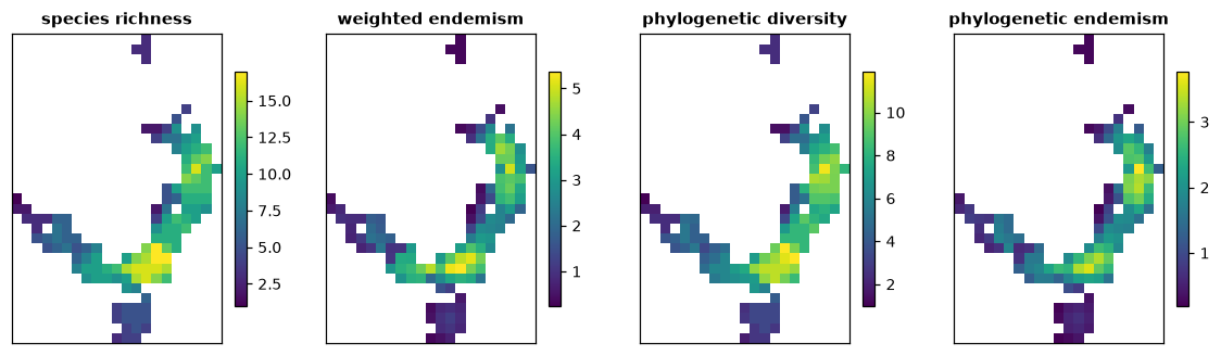
• Richness counts the species of the neighbourhood.
• Weighted endemism (ENDW_WE) adds, for each species, the share of its range inside the neighbourhood: a species found only there counts 1, a widespread one almost nothing.
• Phylogenetic diversity (PD, Faith 1992) is the total length of the branches linking the neighbourhood's species on the tree.
• Phylogenetic endemism (PE_WE, Rosauer et al. 2009) weights each branch by the share of its range in the neighbourhood.

The indices are the same as Biodiverse's, with the same names; ls.bio.list_calculations() lists the 121 calculations and the 282 indices they return. Index values are in res.table (one row per cell) and list indices, such as the endemism weight of each species (res.lists["ENDW_WTLIST"], from endemism_whole_lists), in long tables. res.to_raster("PE_WE") gives a map as an xarray.DataArray and res.to_geodataframe() the cells as polygons.

Neighbourhoods can be any Biodiverse condition: sp_self_only() (the cell alone), sp_block (size => 300000), $D <= 250000, conditions on the coordinates or on group properties. Two conditions give a second neighbour set, used by the indices that compare two sets (turnover, beta diversity).

Is it more than chance? Randomisations and CANAPE

Species-rich cells also tend to have high PD and PE, simply because they have more species. A randomisation redistributes the records while keeping what should not change, and counts how often the random values exceed the observed ones. rand_structured, Biodiverse's default, keeps the richness of every cell and the range size of every species:

rnd = ls.bio.randomise(res, "rand_structured", iterations=999, seed=2024)
p = rnd.p_rank()          # 0.975 or more: higher than chance; 0.025 or less: lower
canape = rnd.canape()
canape["CANAPE_CODE"].value_counts()

CANAPE (categorical analysis of neo- and palaeo-endemism, Mishler et al. 2014) combines the tests of PE and relative PE (phylo_rpe2): cells with significantly high PE are neo-endemism centres when their range-restricted branches are short, palaeo-endemism centres when they are long, mixed otherwise, and super-endemism centres when PE is very highly significant.

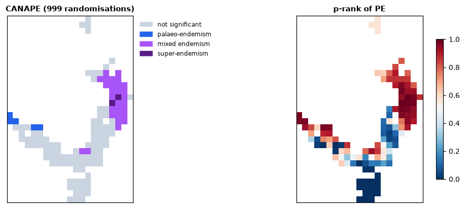
Of the 127 cells, 35 are centres of endemism: 28 mixed, 5 palaeo- and 2 super-endemism centres, mostly in the north-east. The p-ranks show the other side of the test: in the south, PE is lower than chance, as the species there are widespread.

The same seed gives the same randomisations as Biodiverse. rnd.run(900) adds iterations, rnd.comparison() returns Biodiverse's counters and rnd.z_scores() the z-scores. The other randomisations include the swap algorithms (rand_independent_swaps, rand_curveball), spatially structured ones (rand_diffusion, rand_random_walk) and complete spatial randomness (rand_csr_by_group).

Regions: cluster analysis

Clustering joins the cells with the most similar species until one tree remains. The Sorenson dissimilarity with average linkage (UPGMA) is Biodiverse's default; cut gives the regions:

cl = ls.bio.cluster(bd, "SORENSON", "link_average", prng_seed=1)
regions = cl.cut(5)
regions.value_counts()

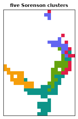
cl.tree is the dendrogram (a Tree; cl.tree.to_newick() for other software) and cl.nodes the values of each join. Other indices include JACCARD, S2, BRAY_CURTIS and PHYLO_SORENSON (with tree=); spatial conditions limit the joins to neighbouring cells (conditions=), giving spatially contiguous regions, and ls.bio.region_grower grows regions that maximise an index.

Saving and exporting

ls.bio.save_session stores basedatas, trees, matrices and results in one file that load_session reads back; to_biodiverse_csv writes a result as Biodiverse's "Delimited text" export does, byte for byte, for scripts and tools that read Biodiverse's tables:

ls.bio.save_session("study.lsbio", sites=bd, tree=tree, indices=res, regions=cl)
res.to_biodiverse_csv("indices.csv")                   # the scalar indices
res.to_biodiverse_csv("endemism_weights.csv", "ENDW_WTLIST")   # a list index

Trees convert to and from Bio.Phylo, DendroPy and ete (tree.to_dendropy(), ls.bio.Tree.from_ete(...)).

Going further

• Group and label properties (read_properties, set_group_properties, set_label_properties) feed the property indices (lbprop_stats, gpprop_stats), with numeric labels such as body sizes or dates (numeric_label_stats, iei_stats).
• Label matrices (read_matrix) give the matrix indices (matrix_stats, mx_rao_qe) and cluster indices from any dissimilarity.
• Phylogenetic community structure: nri_nti_expected_values, phylo_mpd_mntd1 and the net relatedness and nearest taxon indices (Webb et al. 2002).
• Threads: every analysis takes n_threads (default: all cores but one).

The API reference documents every class and function.