Circuit connectivity
Circuit theory models movement across a landscape like electric current through a conductive surface. Every cell has a resistance to movement (low in habitat, high across roads, towns or water); current injected at one place flows to another along all possible routes, most strongly along the easiest ones. The resulting current map shows corridors, pinch points where movement is funnelled, and areas where flow spreads out. Unlike a single least-cost path, it accounts for redundant routes.
You will learn to:
- build a resistance map from land cover;
- map omnidirectional connectivity across a whole landscape (Omniscape);
- compute effective resistances and current between focal points (pairwise);
- inject and ground current where you choose (advanced mode);
- connect each point to all others (one-to-all, all-to-one);
- run existing INI files and networks given as edge lists.
A resistance map
The resistance is a raster of positive values; NaN (or NoData) cells cannot be crossed. A common way to build one is to give each land-cover class a value:
import numpy as np
import landschaft as ls
from landschaft import circuit

landcover = ls.load_raster(ls.example_data("clc"))[:600, :600]   # 15 x 15 km

resistance = ls.reclassify(landcover, [
    (1, 12, 100.0),    # urban, industry, roads: hard to cross
    (12, 23, 20.0),    # agriculture: moderate
    (23, 35, 1.0),     # forest and natural vegetation: easy
    (35, 45, 200.0),   # wetlands and water: very hard
], dtype="float64")
The values are relative: what matters is the ratio between classes. They are usually derived from expert opinion, habitat suitability or movement data.
Omnidirectional connectivity (Omniscape)
Omniscape does not need start and end points. It moves a circular window over the landscape; in every window, current flows from all the sources into the centre. The sum over all windows, the cumulative current, shows how much movement every cell carries between all places within the window's reach.
flow = ls.omniscape(
    resistance,
    radius=30,                 # window radius in cells (750 m)
    block_size=5,              # one window per 5 x 5 block of cells: faster, corrected for artifacts
    flow_potential=True,       # the same with a uniform resistance, for comparison
    normalized_current=True,   # current / flow potential
)
flow
ls.plot(flow)                  # every map on a log scale, over satellite imagery
ls.save(flow, "omniscape_out")  # one GeoTIFF per map, the settings as a table
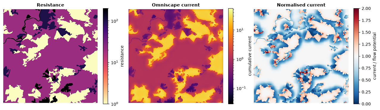
| Output | Meaning |
|---|---|
cum_currmap |
cumulative current: where movement concentrates |
flow_potential |
the current if the whole landscape were equally easy to cross |
normalized_cum_currmap |
their ratio: above 1 = more movement than expected (corridors, pinch points), below 1 = less (impeded) |
By default every cell is a source in proportion to its conductance
(1 / resistance), so habitat both emits and carries movement. Pass
source= for your own source strengths, and r_cutoff= to stop cells above
a resistance from being sources. The radius should reflect the dispersal
distance of the species, in cells.
Speed
The time grows with the number of windows and their size: block_size
of 3–9 cuts the windows by 9–81× with little effect on the result.
Landschaft solves every window exactly and uses all cores but one.
Between focal points (pairwise)
When there are specific places to connect (reserves, populations), mark them on a raster of ids (0 elsewhere) and compute the effective resistance between every pair, and the current that flows between them:
points = np.zeros(resistance.shape)
for k, (row, col) in enumerate([(50, 60), (120, 500), (300, 300), (520, 100), (550, 540)], start=1):
    points[row, col] = k

pairs = circuit.circuitscape_pairwise(resistance, points, cum_map=True)
pairs.resistances
The first row and column hold the point ids; the rest is the effective
resistance between each pair: lower means better connected, through both
shorter and more numerous routes. -1 marks points in parts of the landscape
that are not connected at all.
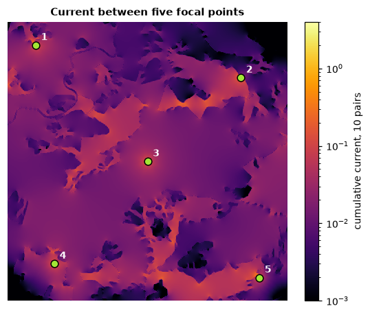
pairs.cum_current sums the current maps of all pairs (numpy arrays on the
resistance's grid); voltage_maps=True and current_maps=True keep the map
of every pair in pairs.maps. Cells of the same id form a focal region
(e.g. a reserve polygon rasterised), treated as a single node.
included_pairs= restricts the pairs to those listed in a file.
Your own sources and grounds (advanced mode)
Inject current where you choose and let it flow to grounds:
source = np.full(resistance.shape, np.nan)
source[50, 60] = 1.0                  # 1 A into this cell
ground = np.full(resistance.shape, np.nan)
ground[550, 540] = 0.0                # a direct ground (0 ohm) here

adv = circuit.circuitscape_advanced(resistance, source, ground)
adv.voltage.max(), adv.current.max()
ground holds resistances to ground (0 is a direct connection, NaN none);
ground_is_resistance=False reads conductances instead. With 1 A injected
and one direct ground, the voltage at the source is the effective resistance
between the two cells.
One-to-all and all-to-one
Each point in turn is connected to all the others (all_to_one=True: all
the others inject into it). The table gives, per point, the resistance
between it and the rest; cum_map=True sums the current maps.
Existing projects and networks
INI files of existing projects run as they are, and write the same output files:
circuit.circuitscape_ini("my_project.ini")   # raster or network, any mode
circuit.omniscape_ini("my_omniscape.ini")
Networks given as edge lists (node, node, resistance) instead of rasters:
edges = [[1, 2, 2.0], [2, 3, 1.0], [1, 3, 4.0], [3, 4, 1.5]]
net = circuit.circuitscape_network_pairwise(edges, [1, 4])
net.resistances
circuitscape_network_advanced(edges, sources, grounds) is the advanced mode
on a network.
Good practice
- Choose the radius (Omniscape) or the points (pairwise) from the ecology of the species, and test how sensitive the results are to the resistance values.
- Keep NoData to cells that truly cannot be crossed; use high resistances for strong barriers that are still crossable.
- Large maps: Omniscape's memory grows with the window size;
memory_limit=caps it (fewer windows at once).
Next steps
- Cost distances and single best routes: distance & restoration.
- Patch-based networks: habitat networks.