Chapter 6

Landscape connectivity

Habitat that cannot be reached is of little use. A woodland isolated by kilometres of cropland may never be colonised by a forest beetle; a population cut off from its neighbours loses genetic diversity and cannot be rescued after a bad year. Connectivity, the ease with which organisms move between the parts of a landscape, links the pattern of the previous chapters to the processes of dispersal, gene flow and range shifts. This chapter introduces the concepts; chapters 7, 8 and 9 present the three families of models.

In this chapter

• what connectivity is: structural, functional, potential and actual;
• dispersal and dispersal kernels;
• resistance surfaces: how the matrix is turned into a cost of movement;
• cost distance versus straight-line distance;
• the families of connectivity models and the assumptions of each.

What connectivity is

The classic definition is the degree to which the landscape facilitates or impedes movement among resource patches (Taylor et al., 1993). Two properties follow from it. Connectivity is a property of the landscape, not only of the habitat: the land between patches matters. And it is species-specific: the same hedge that connects woodlands for a dormouse is irrelevant for a bat and invisible for a deer.

Three distinctions organise the literature (Tischendorf & Fahrig, 2000; Calabrese & Fagan, 2004):

Kind	Based on	Example measure
structural	the physical arrangement of habitat only	distance to the nearest patch, presence of corridors, MSPA bridges
potential	structure plus limited knowledge of the organism (a dispersal distance, a resistance to movement)	graph indices with a dispersal kernel, cost distances, circuit models
actual (realised)	observed movement	tracking, mark–recapture, gene flow

Structural connectivity is easy to map but says nothing on whether an organism actually moves; actual connectivity is what matters but is costly to measure and specific to a place and time. Most applied work uses potential connectivity: models that combine the map with a few, well-chosen facts about the species. All the connectivity tools of Landschaft are of this kind. Their results are hypotheses about movement, to be tested with movement or genetic data when possible (Bélisle, 2005).

Dispersal

Dispersal is any movement that can lead to gene flow: from the place of birth to the place of breeding, or between breeding places. It has three stages, emigration, transfer and immigration, each influenced by the landscape (Bowler & Benton, 2005). Connectivity models focus on the transfer stage: how far organisms go and which routes they take.

A dispersal kernel describes the probability of moving a given distance. The simplest and most used in connectivity indices is the negative exponential:

p(d) = e^{−k d},     with k = −ln(p₀) / d₀ p(d): probability of covering distance d; k is set so that the probability at a reference distance d₀ is p₀, for instance p₀ = 0.5 at the median dispersal distance.

import numpy as np
import pandas as pd

median_dispersal = 1000.0                       # metres: half the dispersers go further
k = -np.log(0.5) / median_dispersal
distances = np.array([0, 250, 500, 1000, 2000, 4000, 8000])
pd.DataFrame({"distance (m)": distances, "p(d)": np.exp(-k * distances).round(3)})

Each doubling of the distance squares the probability: 0.5 at 1 km, 0.25 at 2 km, 0.06 at 4 km. The kernel is a statement about the species, calibrated from telemetry, mark–recapture or allometric relations with body size, and it matters most in its tail: rare long-distance dispersal events drive colonisation and range expansion (Nathan, 2006). When the kernel is uncertain, analyse several distances (chapter 2).

Resistance surfaces

Straight-line distance treats all land between patches as equally easy to cross, which it rarely is. A resistance surface assigns every cell a value proportional to the cost, energy, risk or reluctance of crossing it (Zeller et al., 2012). Movement models then measure distances in units of accumulated resistance rather than metres.

Resistance values come from three sources, from weakest to strongest (Spear et al., 2010; Zeller et al., 2012):

1. Expert opinion: ranks of land-cover classes from literature and experience. Fast, but subjective and hard to validate.
2. Habitat suitability: resistance as a decreasing function of a habitat model's suitability. A negative exponential transformation, which keeps resistance low across most of the good habitat and rises steeply in poor habitat, often performs better than a linear one (Keeley et al., 2016).
3. Movement or genetic data: resistance values that best explain observed paths, telemetry locations or genetic distances between populations.

Resistance values are relative: what matters is the ratio between classes. Report how they were obtained and test how sensitive the results are to them, for example by halving and doubling the contrast between habitat and matrix.

Try it: cost distance versus straight-line distance

Build a resistance surface for a forest species from land cover (forest and semi-natural areas easy to cross, farmland ten times harder, built-up land fifty times, water a hundred times), then measure, from every cell, the distance to the nearest forest in both ways:

from scipy import ndimage
import landschaft as ls

landcover = ls.load_raster(ls.example_data("clc"))[:800, :800]   # 20 x 20 km

resistance = ls.reclassify(landcover, [(1, 12, 50.0),     # artificial surfaces
                                       (12, 23, 10.0),    # agricultural areas
                                       (23, 35, 1.0),     # forest and semi-natural areas
                                       (35, 45, 100.0)],  # wetlands and water
                           dtype="float64")

forest = np.isin(landcover.values, [23, 24, 25])
euclidean_m = ndimage.distance_transform_edt(~forest) * 25          # metres
cost_m = np.asarray(ls.cost_distance(resistance, forest)) * 25      # metres x resistance

cost_distance accumulates, along the cheapest route from the sources, the resistance of each step times its length in cells; multiplying by the cell size expresses it in "resistance-weighted metres": the length of the route if all of it had resistance 1. Now compare the cells that lie about 1 km from the nearest forest:

ring = (euclidean_m > 950) & (euclidean_m < 1050)
pd.Series(cost_m[ring] / 1000).describe(percentiles=[0.05, 0.5, 0.95]).round(1)

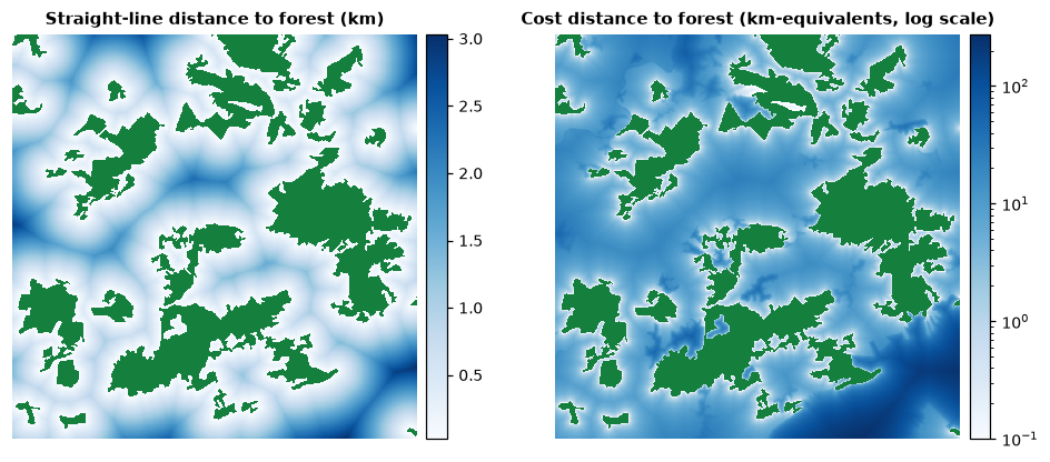
All these cells are 1 km from forest as the crow flies, yet their cost distances range from about 9 to more than 100 km-equivalents: across farmland a forest species pays about ten times the straight-line distance, across towns and water far more. Two places at the same distance from habitat can be very differently connected to it, which is the whole point of resistance-based models.

The families of connectivity models

Family	The landscape is...	Movement is assumed to...	Answers	Chapter
simple indices	patches and distances	–	how isolated is each patch? (enn, proximity)	5
graphs	nodes (patches) and links (distances or probabilities)	depend on the distance between patches, via a threshold or a kernel	how much habitat is reachable? which patches and links matter?	7
circuits	a conductive surface	follow random walks: every route used, in proportion to its ease	where does movement concentrate? where are pinch points and barriers?	8
least-cost	a cost surface	follow the single cheapest route, with full knowledge of the landscape	what is the best corridor between two areas, and what does it cost?	9

The families are complementary rather than competing (McRae et al., 2008; Kindlmann & Burel, 2008). Graphs summarise connectivity at the level of patches and are ideal for ranking conservation priorities; least-cost paths give a single, easily mapped corridor, but assume an animal that knows the whole landscape; circuits consider all routes and highlight bottlenecks, assuming an animal that knows nothing beyond its next step. Real behaviour lies somewhere in between. A robust conclusion is one that holds across more than one model.

Key points

• Connectivity is a property of the whole landscape and of a species; it can be structural, potential or actual.
• Dispersal kernels express how the probability of movement decreases with distance; their tail matters.
• Resistance surfaces translate the matrix into a cost of movement; their values are relative, should be justified and should be tested.
• Cost distance can differ from straight-line distance by an order of magnitude.
• Graph, circuit and least-cost models make different assumptions about movement and answer different questions.

Check your understanding

1. A map shows that two reserves are linked by an MSPA bridge. What kind of connectivity does that establish, and what is still unknown?
2. With a negative exponential kernel of p = 0.5 at 500 m, what is the probability of crossing 1.5 km?
3. Why should resistance values be tested with a sensitivity analysis?

Answers

1. Structural connectivity. Whether the species can and does move along the bridge (its width, its quality, the species' behaviour) is unknown: that is functional or actual connectivity.
2. 1.5 km is three times 500 m, so p = 0.5³ = 0.125.
3. Because they are usually uncertain (often from expert opinion), and the location of corridors and the ranking of patches can change with them. Conclusions that survive a range of plausible values are more credible.

References

• Bélisle, M. (2005). Measuring landscape connectivity: the challenge of behavioral landscape ecology. Ecology, 86(8), 1988–1995.
• Bowler, D. E., & Benton, T. G. (2005). Causes and consequences of animal dispersal strategies: relating individual behaviour to spatial dynamics. Biological Reviews, 80(2), 205–225.
• Calabrese, J. M., & Fagan, W. F. (2004). A comparison-shopper's guide to connectivity metrics. Frontiers in Ecology and the Environment, 2(10), 529–536.
• Keeley, A. T. H., Beier, P., & Gagnon, J. W. (2016). Estimating landscape resistance from habitat suitability: effects of data source and nonlinearities. Landscape Ecology, 31, 2151–2162.
• Kindlmann, P., & Burel, F. (2008). Connectivity measures: a review. Landscape Ecology, 23, 879–890.
• McRae, B. H., Dickson, B. G., Keitt, T. H., & Shah, V. B. (2008). Using circuit theory to model connectivity in ecology, evolution, and conservation. Ecology, 89(10), 2712–2724.
• Nathan, R. (2006). Long-distance dispersal of plants. Science, 313(5788), 786–788.
• Spear, S. F., Balkenhol, N., Fortin, M.-J., McRae, B. H., & Scribner, K. (2010). Use of resistance surfaces for landscape genetic studies: considerations for parameterization and analysis. Molecular Ecology, 19(17), 3576–3591.
• Taylor, P. D., Fahrig, L., Henein, K., & Merriam, G. (1993). Connectivity is a vital element of landscape structure. Oikos, 68(3), 571–573.
• Tischendorf, L., & Fahrig, L. (2000). On the usage and measurement of landscape connectivity. Oikos, 90(1), 7–19.
• Zeller, K. A., McGarigal, K., & Whiteley, A. R. (2012). Estimating landscape resistance to movement: a review. Landscape Ecology, 27, 777–797.