Chapter 11

Continuous surfaces¶

Every chapter so far looked at landscapes through categorical maps: habitat or not, forest or pasture, patches with sharp edges. Much of what shapes organisms is not categorical at all. Canopy height, greenness, soil moisture, temperature and elevation change gradually, and a forest thinning into woodland has no edge to draw. This chapter treats the landscape as a surface: a continuous variable measured in every cell, described by how it varies rather than by the patches a threshold would cut out of it.

In this chapter

the patch-mosaic and the gradient models of landscape structure, and what a threshold does to a continuous map;
surface metrics: amplitude, height distribution, slopes and features, computed by hand on a tiny surface;
the bearing area curve;
the spatial structure of a surface: autocorrelation, anisotropy, direction, wavelength, fractal dimension;
surfaces in moving windows, and terrain indices of elevation models;
summits, saddles and the hilltops protected by Brazil's Forest Code;
the gravity model of spatial interaction;
pitfalls in measuring surfaces.

Patches or gradients?¶

The patch-mosaic model, on which landscape metrics rest (chapter 5), sees a landscape as discrete, internally uniform patches with abrupt boundaries. It fits many human-shaped landscapes: a field ends at a fence. The gradient model (McGarigal & Cushman, 2005) sees structure as continuous variation in space, of which patches are a special case. It fits variables that change gradually, and the way organisms respond to many of them: a bird does not switch from forest to non-forest at 60 % canopy cover.

Turning a continuous variable into patches needs a threshold, and the threshold is rarely given by the ecology. The patch structure can depend on it more than on the landscape:

import numpy as np
import landschaft as ls

ndvi = ls.load_raster(ls.surface.example_data("orforest"))
for t in (0.60, 0.65, 0.70, 0.75):
    habitat = np.where(ndvi.values >= t, 2, 1).astype("uint8")
    m = ls.Landscape(habitat).class_metrics(["pland", "np"]).set_index("class").loc[2]
    print(f"NDVI >= {t:.2f}: {m['pland']:5.1f} % habitat in {int(m['np']):5d} patches")

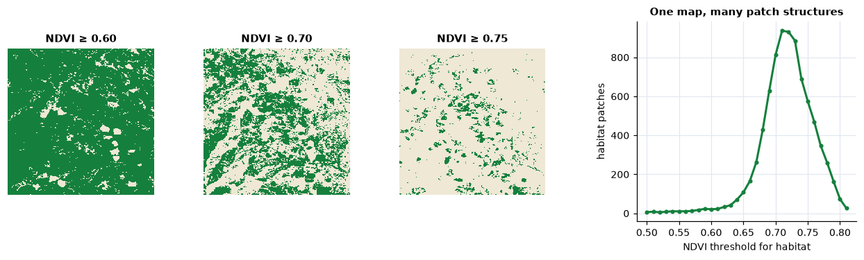
The same NDVI map as habitat at three thresholds, and the number of patches

At NDVI 0.60 the "forest" covers 92 % of the map in 21 patches; at 0.70 it covers 42 % in 814 patches, at 0.75 only 9 % in 574. Nothing in the landscape changed: only the threshold. Surface metrics describe the map without choosing one (McGarigal et al., 2009).

The reference surface¶

Surface metrics come from the measurement of engineered surfaces, where roughness is measured as deviations from a reference plane; they are standardised as ISO 25178. In a landscape the reference is the broad trend of the variable: a gradient of greenness from one side of the map to the other is not texture. The first step is therefore to remove it, fitting a polynomial surface in the coordinates and keeping the residuals:

z = ls.surface.remove_plane(ndvi)       # residuals from the best polynomial of order 0-3
print(z.attrs["order"], round(float(z.mean()), 12))

Everything that follows describes z, heights above (positive) and below (negative) the trend.

Surface metrics by hand¶

A tiny surface of 4 × 4 cells is enough to see the main metrics:

toy = np.array([[ 0.2, -0.1,  0.0,  0.3],
                [-0.4,  0.1,  0.5, -0.2],
                [ 0.1, -0.3,  0.2,  0.0],
                [ 0.0,  0.4, -0.2, -0.6]])
dev = toy - toy.mean()

Amplitude¶

The average roughness Sa and the root mean square roughness Sq measure how far the surface strays from its mean:

Sa = (1/N) Σ |z_i − z̄| Sq = √[ (1/N) Σ (z_i − z̄)² ] N: number of cells with a value; z̄: their mean. Sq weights large deviations more than Sa.

by_hand = {"Sa": np.abs(dev).mean(), "Sq": np.sqrt((dev ** 2).mean())}
tool = ls.surface.metrics(toy, ["sa", "sq"])
print(by_hand, tool.to_dict())

The shape of the height distribution¶

Two surfaces with the same Sq can look very different. The skewness Ssk and the kurtosis Sku describe the distribution of heights:

Ssk = (1/Sq³) (1/N) Σ (z_i − z̄)³ Sku = (1/Sq⁴) (1/N) Σ (z_i − z̄)⁴ − 3 Ssk < 0: deep valleys in a plateau (a closed forest with clearings); Ssk > 0: peaks above a plain (scattered trees in grassland). Sku > 0: a peaked distribution with long tails, a few extreme cells; Sku = 0 for a normal distribution.

sq = np.sqrt((dev ** 2).mean())
g1 = (dev ** 3).mean() / sq ** 3
print(g1, ls.surface.ssk(toy, adj=False))
print((dev ** 4).mean() / sq ** 4 - 3, ls.surface.sku(toy))

ssk by default multiplies by √(N(N−1))/(N−2), the adjusted coefficient that corrects the bias of small samples.

Slopes and features¶

Sdq, the root mean square slope, averages the squared height differences between each cell and its right and lower neighbours; Sdr compares the area of the surface, triangulated between cell centres, with the area of its footprint. Peaks are cells higher than their eight neighbours (and than the reference plane); Sds is their density:

right = toy[:-1, :-1] - toy[:-1, 1:]
down = toy[:-1, :-1] - toy[1:, :-1]
print(np.sqrt((right ** 2 + down ** 2).mean()), ls.surface.sdq(toy))
print(ls.surface.find_peaks(toy))

On the 4 × 4 surface only the four inner cells can be peaks, and one is: 0.5, above all eight neighbours.

The bearing area curve¶

Sort the heights from the highest and plot, for each, the share of the surface at or above it: this is the bearing area curve (Abbott-Firestone curve). Its top shows the peaks, its bottom the valleys, and its middle, the core, the bulk of the surface. A straight line fitted to the flattest 40 % of the curve separates the core (height range Sk) from the peaks above it (Spk) and the valleys below it (Svk). The void volumes between the curve and its top measure how much "room" the core and the valleys leave (Sci, Svi).

curve = ls.surface.bearing_area(toy)
print(curve)
print(ls.surface.height_ba(toy, 0.5))     # the height with half the surface above it

On a forest's greenness, a long valley tail (large Svk) means a closed canopy with deep, rare gaps; a long peak tail (large Spk), scattered crowns rising above a lower canopy.

Spatial structure¶

The metrics above ignore where the heights are: shuffling the cells leaves them unchanged, as composition metrics are unchanged by shuffling (chapter 5). Spatial metrics look at arrangement.

The areal autocorrelation function (aacf) gives, for every lag (a shift in x and y), how similar the surface is to itself shifted by that lag: 1 at zero lag, falling with distance. The autocorrelation length Sal is the shortest distance at which it drops to 0.2: the size of the "grain" of the texture (chapter 2).
The texture aspect ratio Str divides the shortest decay length by the longest: near 1 for an isotropic surface (the same in every direction), near 0 for a surface stretched in one direction, like ridges and valleys or rows of trees.
The Fourier spectrum decomposes the surface into waves. Summing its amplitude by angle gives the dominant direction of the texture (Std), by radius the dominant frequency (Srw, a radius in the spectrum: the number of repetitions across the map, times the cell size).
The fractal dimension Sfd, between 2 (a smooth surface) and 3 (a surface so rough that it fills space), measures how fast the surface area grows as it is measured with finer cells (Clarke, 1986).

field = ls.nlm.gaussian_field(120, 120, autocorr_range=15, seed=1)
x = np.arange(120)
ridges = np.sin(2 * np.pi * x / 12)[None, :] + 0.3 * field.values
for name, s in (("isotropic field", field), ("ridges", ridges)):
    lengths = ls.surface.scl(s)
    print(f"{name:16s} Sal {lengths[0]:5.1f}  Str {ls.surface.stxr(s)[0]:.2f}  "
          f"Std {ls.surface.std(s)[0]:5.1f}  Srw {ls.surface.srw(s)[0]:5.1f}")

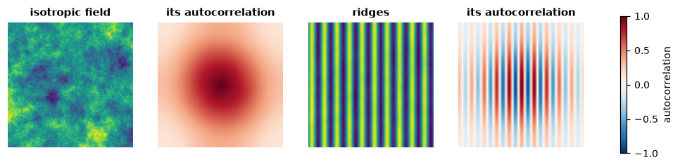
Two surfaces and their autocorrelation

The Gaussian field decays at about the same rate in every direction (Str 0.73); the ridges stay correlated along their length and alternate across it, which shows as a short Sal (3 cells, a quarter of their period), a low Str (0.04), a direction of 0 degrees (the texture varies along x) and an Srw of about 10: the ridges repeat 10 times across the 120 cells, a wavelength of 120 / 10 = 12 cells.

Surfaces in moving windows¶

A single value per map hides where the surface is rough and where it is smooth. Computing a metric in a window around every cell gives a texture image, a map of heterogeneity that can enter a species distribution model like any other covariate. The window size is the scale of the analysis (chapter 2): choose it from the organism's perceptual range or home range, not from the map.

texture = ls.surface.window_metrics(z, ["sa", "sku"], window=9)
print(float(texture["sa"].mean()), float(texture["sku"].mean()))

Elevation: terrain indices¶

A digital elevation model (DEM) is the most common surface of all, and terrain has indices of its own, many of them designed with ecology in mind:

Slope and aspect, from the height differences of the 3 × 3 neighbourhood (Horn, 1981).
Topographic position index (TPI; Weiss, 2001): the elevation minus the mean of a window. Positive on ridges and hilltops, negative in valleys and hollows, near 0 on flats and even slopes; with windows of several sizes it separates small hollows from large valleys. The hierarchical slope position (hsp; Murphy et al., 2010) sums it over scales.
Ruggedness: the terrain ruggedness index (TRI; Riley et al., 1999) from the elevation differences with the neighbours, the vector ruggedness measure (VRM; Sappington et al., 2007) from the dispersion of the surface's orientation, so that a steep but even slope is not rugged.
Curvature (Zevenbergen & Thorne, 1987): profile curvature along the slope (accelerating or slowing flow), planform curvature across it (converging or diverging flow).
Heat load (McCune & Keon, 2002): potential solar radiation from slope, aspect and latitude, the warm south-west slopes of the northern hemisphere against the cool north-east ones; trasp is a simpler transformation of aspect (Roberts & Cooper, 1989).

The TPI of a cell is easy to check by hand:

dem = ls.load_raster(ls.surface.example_data("orelevation"))
tpi = ls.surface.tpi(dem, 3)
window = dem.values[99:102, 199:202]
print(dem.values[100, 200] - window.mean(), float(tpi.values[100, 200]))

Summits, saddles and protected hilltops¶

A DEM is also a set of elevations: summits, each standing above a base. Where is the base of a hill? Walking down from a summit, its region grows until it meets the region of a higher summit at a saddle (a col): below that level the two are one landform. The height of the saddle under a summit that leads to higher ground is the summit's key col, and the summit's height above it its topographic prominence. The highest summit of an area has no higher neighbour: its base is the lowest ground around it, a plain, a river or the sea.

The definition matters in law. Brazil's Forest Code (Lei 12.651/2012, art. 4, IX) protects the tops of hills, mountains and ranges at least 100 m high and with a mean slope above 25°: the area above the contour at two thirds of the height, measured from the base, which is the adjacent plain or water body or, in undulating relief, "the nearest saddle point". These hilltop permanent protection areas (APP de topo de morro) keep vegetation on the steep upper slopes, where clearing causes erosion and landslides.

ls.surface.hilltop sweeps the cells from the highest down, joining each to its swept neighbours, and records each summit's base where its region meets a higher one (or the plain, given as a mask). Two cones that meet at a saddle show it:

yy, xx = np.mgrid[0:60, 0:100] * 30.0 + 15                  # 30 m cells
big = 500 + np.clip(400 - np.hypot(yy - 885, xx - 1065), 0, None)
small = 500 + np.clip(250 - np.hypot(yy - 885, xx - 1545), 0, None)
cones = np.maximum(big, small)                              # 45 degree slopes on a plain at 500 m
h = ls.surface.hilltop(cones, extent=(0, 3000, 0, 1800))
hills = h.hills[h.hills.height > 0]
print(hills[["top", "base", "base_kind", "height", "mean_slope", "threshold"]].round(1))
print(cones[29, 35:52].min())                               # the lowest point of the ridge between them

The big cone stands 400 m above the plain; the small one 150 m above the saddle at 600 m, the lowest point of the ridge that joins them, not above the plain. Both qualify, and each protects the area above its threshold: 766.7 m and 700 m. With the older rule of CONAMA 303/2002, hills of 50 m and a slope of 30 % along the line of steepest slope also count: min_height=50, min_slope=16.7, slope="line".

Spatial interaction: the gravity model¶

Towns, markets and ports pull activity towards them, more the larger they are and the closer. The gravity model of spatial interaction (Haynes & Fotheringham, 1984) sums that pull over the sources:

P_i = Σ_k m_k / d_ik^β m_k: the mass of source k (population, production); d_ik: its distance from cell i; β: the distance decay (2: the inverse square).

The potential is a common driver of land change: deforestation and urbanisation follow it. ls.surface.gravity computes it, with distances in cells (a source's own cell at 1, as Dinamica EGO does) or in map units, and ls.simulate.gravity_of recomputes it from the simulated map at every step (chapter 14). By hand, for the cell of the smaller of two towns:

towns = np.full((5, 7), np.nan)
towns[1, 1], towns[3, 5] = 2000, 500                        # populations
p = ls.surface.gravity(towns, 2)
print(2000 / ((3 - 1) ** 2 + (5 - 1) ** 2) + 500 / 1, float(p[3, 5]))

Pitfalls¶

Remove the trend deliberately. Metrics of a surface with a trend mostly measure the trend. remove_plane chooses the order of the polynomial by BIC; if the trend is ecologically meaningful (an elevation gradient), decide whether it is part of what you want to measure.
Units. Amplitude metrics are in the units of the variable; slopes in units per cell; Sal and Srw in map units (metres on longitude/latitude rasters). Sdr and Ssc are computed on heights rescaled to 0–1, so they compare surfaces measured in different units.
Noise is roughness. Sensor noise, clouds and stripes in imagery add to Sa, Sdq and the fractal dimension. Smooth or mask them first, and compare maps from the same sensor and processing.
Resolution. Like landscape metrics, surface metrics depend on the grain (chapter 2): slopes and roughness in particular. Compare maps at the same resolution.
Redundancy. Sa and Sq, or Sdq and Sdr, are strongly correlated; a handful from different families (amplitude, distribution, spatial) says most of what the full set says, as with patch metrics (chapter 5).
Hilltops depend on the DEM. Bases, heights and mean slopes change with the resolution and the errors of the elevation model (a coarse DEM flattens slopes and can drop a hill below 25°), and on what is given as plain or water. Automatic delineation is a starting point for field and legal work, not its end.
Edges and missing cells. Windows that reach the edge of the map or a missing cell give missing values (or, for the Fourier metrics, use the largest square without missing cells).

Key points

Continuous variables need not be thresholded: surface metrics describe them directly, and thresholds can change patch structure more than the landscape does.
Remove the trend, then describe amplitude (Sa, Sq), the height distribution (Ssk, Sku, the bearing area curve), slopes and features (Sdq, Sdr, Sds) and spatial structure (Sal, Str, Std, Srw, Sfd).
Texture images map heterogeneity at a chosen scale.
Terrain indices (TPI, TRI, VRM, curvature, heat load) turn a DEM into ecologically meaningful variables.
A summit's base is the saddle where it meets higher ground, or the plain; the protected hilltop is the area above two thirds of its height.

Check your understanding¶

Two forests have the same Sq of NDVI residuals, but one has Ssk = −2 and the other Ssk = +2. Describe each canopy.
Why does the number of habitat patches in the NDVI example change so much between thresholds 0.60 and 0.75?
A surface has a texture aspect ratio (Str) of 0.05. What does it look like, and which metric tells its orientation?
A peak of 1000 m stands on a range whose highest summit is 1100 m; the lowest point of the ridge between them is at 960 m and the range rises from a plain at 300 m. What is the peak's height for the Forest Code, and is it a protected hill?

Answers

Ssk = −2: most cells are slightly above the mean, with rare, deep lows: a closed canopy with a few gaps or clearings. Ssk = +2: most cells slightly below the mean, with rare high cells: an open canopy with scattered dense crowns.
Most cells lie between those values: the threshold cuts through the bulk of the height distribution, so small changes of threshold move many cells across it, splitting and merging patches. The landscape did not change; the definition of habitat did.
Strongly anisotropic: stretched in one direction, like ridges, valleys or rows. The texture direction Std gives the orientation (and the wavelength Srw the spacing of the ridges).
Its base is the saddle at 960 m, where it meets the higher summit: 40 m, below the 100 m the law asks, so it is not a hill of its own. It is part of the range, whose highest summit stands 800 m above the plain; if that qualifies, its protected area starts at 300 + 2/3 × 800 ≈ 833 m, and the peak, joined to the summit by a ridge that never drops below 960 m, lies inside it.

References¶

Clarke, K. C. (1986). Computation of the fractal dimension of topographic surfaces using the triangular prism surface area method. Computers & Geosciences, 12(5), 713–722.
Brasil (2012). Lei nº 12.651, de 25 de maio de 2012 (Código Florestal), art. 4, IX. Diário Oficial da União, 28 May 2012.
CONAMA (2002). Resolução nº 303, de 20 de março de 2002. Conselho Nacional do Meio Ambiente, Brasília.
Haynes, K. E., & Fotheringham, A. S. (1984). Gravity and Spatial Interaction Models. Sage, Beverly Hills.
Horn, B. K. P. (1981). Hill shading and the reflectance map. Proceedings of the IEEE, 69(1), 14–47.
ISO 25178-2 (2012). Geometrical product specifications (GPS) — Surface texture: Areal — Part 2: Terms, definitions and surface texture parameters. International Organization for Standardization.
McCune, B., & Keon, D. (2002). Equations for potential annual direct incident radiation and heat load. Journal of Vegetation Science, 13(4), 603–606.
McGarigal, K., & Cushman, S. A. (2005). The gradient concept of landscape structure. In J. A. Wiens & M. R. Moss (Eds.), Issues and Perspectives in Landscape Ecology (pp. 112–119). Cambridge University Press.
McGarigal, K., Tagil, S., & Cushman, S. A. (2009). Surface metrics: an alternative to patch metrics for the quantification of landscape structure. Landscape Ecology, 24, 433–450.
Murphy, M. A., Evans, J. S., & Storfer, A. (2010). Quantifying Bufo boreas connectivity in Yellowstone National Park with landscape genetics. Ecology, 91(1), 252–261.
Riley, S. J., DeGloria, S. D., & Elliot, R. (1999). A terrain ruggedness index that quantifies topographic heterogeneity. Intermountain Journal of Sciences, 5(1–4), 23–27.
Roberts, D. W., & Cooper, S. V. (1989). Concepts and techniques of vegetation mapping. In Land Classifications Based on Vegetation: Applications for Resource Management (pp. 90–96). USDA Forest Service General Technical Report INT-257.
Sappington, J. M., Longshore, K. M., & Thompson, D. B. (2007). Quantifying landscape ruggedness for animal habitat analysis: a case study using bighorn sheep in the Mojave Desert. Journal of Wildlife Management, 71(5), 1419–1426.
Smith, A. C., Dahlin, K. M., Record, S., Costanza, J. K., Wilson, A. M., & Zarnetske, P. L. (2021). The geodiv R package: tools for calculating gradient surface metrics. Methods in Ecology and Evolution, 12(11), 2094–2100.
Weiss, A. D. (2001). Topographic position and landforms analysis. Poster presentation, ESRI User Conference, San Diego, CA.
Zevenbergen, L. W., & Thorne, C. R. (1987). Quantitative analysis of land surface topography. Earth Surface Processes and Landforms, 12(1), 47–56.