Chapter 12.8

Management actions¶

Protecting land is one conservation action among many. In most landscapes biodiversity is lost to threats: deforestation, fire, invasive species, overgrazing, pollution. Fighting a threat where it harms the most species can achieve more than buying land where nothing threatens them. Multi-action planning decides which action to take where: protect here, fight fire there, restore elsewhere, at the least cost or with the most benefit (Cattarino et al. 2015; Salgado-Rojas et al. 2020).

In this chapter

threats, actions, sensitivity and benefit: the vocabulary of multi-action planning;
a multi-action plan for Serra Verde's deforestation and fire;
recovery and conservation targets, and maximizing benefit with a budget;
response curves: how features respond to threats and to their removal;
dependencies between places, such as along a river;
inputs as tables, for any planning units;
zones of management, and when to use zones, actions or restoration.

From places to actions¶

The problems of the previous chapters choose places. A multi-action problem chooses actions in places:

Ingredient	Meaning	In Serra Verde
planning units	the places, each with a cost of monitoring (managing it at all)	the 4825 cells, with the land cost
features	what should benefit	the eight species and habitats
threats	what harms the features, with an intensity in every unit	deforestation along roads and around cities; fire in a band across the west
actions	one per threat: removing it from a unit, at a cost	fighting deforestation (30 per cell) and fire (10 per cell)
sensitivity	which features each threat harms, and how much	by default every feature to every threat

The benefit of a unit for a feature then has two parts (Salgado-Rojas et al. 2020):

conservation: the feature's amount in a monitored unit that no threat harms. Being managed is enough to keep it;
recovery: the amount that comes back when the threats that harm it are removed by actions.

Targets can be set for each: so much recovered, so much conserved.

In plain words

Think of a doctor with a limited budget for a population of patients. Some are healthy and only need a check-up (conservation). Others are ill and need a specific treatment (an action against a threat). Treating the wrong illness, or treating patients who would recover anyway, wastes the budget. Multi-action planning matches treatments to patients.

A plan against deforestation and fire¶

The threats of Serra Verde come with the example data. actions_raster_data turns rasters of costs, features and threats into the inputs of a multi-action problem:

import numpy as np
import pandas as pd
import landschaft as ls

P = ls.prioritize
cost = ls.load_raster(P.example_data("cost"))
features = ls.load_raster(P.example_data("features"))
threats = ls.load_raster(P.example_data("threats"))     # bands: deforestation, fire (intensity 0-1)

d = P.actions_raster_data(cost, features, threats, action_cost=[30, 10],
                          target_recovery=0.3, target_conservation=0.1)
print(d.n_units, "planning units,", d.n_actions, "possible actions")

Each unit where a threat occurs is a possible action. The targets ask for 30 % of each feature's threatened amount to be recovered and 10 % of its unthreatened amount to be conserved. minimizeCosts meets them at the least total cost of monitoring and actions:

sol = d.problem("minimizeCosts").add_highs_solver(gap=0.01).solve()
print(sol.status, f"total cost {sol.objective:,.0f}")
sol.cost()                      # monitoring, then every threat's actions

b = sol.benefit()
b["feature"] = [str(n) for n in features.band.values]
b.round(1)

Threats and a multi-action plan — Left and middle: the intensity of deforestation (along the highway and around the cities) and of fire (a band across the west). Right: the plan. Fire is fought in large blocks of the western forests, where it threatens the jaguar, the harpy eagle and the araucaria forest. Deforestation is fought along the coast and around the cities, where it threatens the mangrove and the tamarin. A few cells (light green) are only managed, to conserve features no threat harms there.

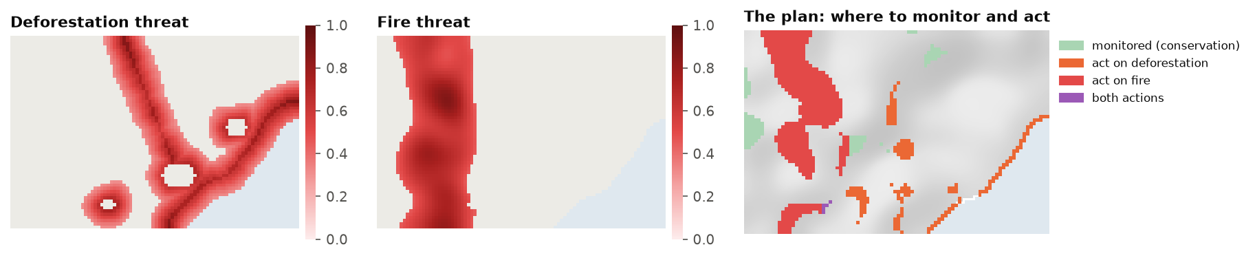
sol.maps() returns the plan as rasters (a band for monitoring, one per threat), and sol.action_summary() as a table of every unit's actions. ls.plot(sol) draws it.

With a budget¶

When the money is fixed, maximizeBenefits finds the plan with the most total benefit within it:

best = d.problem("maximizeBenefits", budget=20_000).add_highs_solver(gap=0.01).solve()
b = best.benefit()
b["feature"] = [str(n) for n in features.band.values]
b[["feature", "benefit.conservation", "benefit.recovery"]].round(1)

Like maximum utility (chapter 12.4), maximizing total benefit favours widespread features: here the tamarin and the mangrove get nothing, and the tapir almost nothing. Benefits are added up in each feature's own units, so a widespread feature always offers more benefit per dollar. Targets (with minimizeCosts), or features scaled to comparable totals, are the remedies.

How features respond¶

How much does a feature suffer from a threat, and how much does it gain when the threat is removed? Two curves answer it.

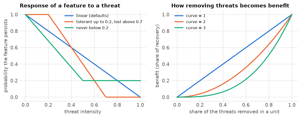
Sensitivity. A feature's probability of persisting falls as the intensity of a threat grows. The sensitivity table (feature, threat and the four parameters delta1 to delta4) shapes this response. By default it is a straight line from full persistence with no threat to none at the strongest threat. A feature can also tolerate a threat up to some intensity, or never be lost entirely.

Curve. How the removal of threats in a unit turns into benefit. With curve=1, benefit grows in proportion to the share of the threats removed; with curve=2 or 3, half the threats removed gives a quarter or an eighth of the benefit. Partial action is worth little, and the plan prefers to remove all the threats from fewer units.

Sensitivity and response curves — Left: three sensitivities of a feature to a threat, set by `delta1` to `delta4`: linear (the default), tolerant up to an intensity of 0.2 and lost above 0.7, and never falling below 0.2. Right: the benefit of removing a share of the threats from a unit, with `curve` 1, 2 and 3.

sens = pd.DataFrame({"feature": ["mangrove", "golden_lion_tamarin"], "threat": ["deforestation"] * 2,
                     "delta1": [0.0, 0.1], "delta2": [0.5, 0.6], "delta3": [0.0, 0.0], "delta4": [1.0, 1.0]})
d2 = P.actions_raster_data(cost, features, threats, action_cost=[30, 10], sensitivity=sens,
                           target_recovery=0.3, target_conservation=0.1)
s2 = d2.problem("minimizeCosts").add_highs_solver(gap=0.01).solve()
print(f"only the mangrove and the tamarin, and only to deforestation: {s2.objective:,.0f}")

When a sensitivity table is given, only its pairs count: here the mangrove and the tamarin are harmed by deforestation, and the other features by nothing, so for them only conservation targets apply.

Dependencies between places¶

In a river, what happens upstream reaches every place downstream. Managing a reach whose upstream reaches are left degraded wastes money. add_directional_dependencies expresses this. Its flow table pairs each unit (target_pu) with the unit it depends on (source_pu). Managing the target without its source then either costs a penalty (soft) or is not allowed (hard=True):

# every river cell depends on the river cell just upstream of it (higher elevation)
flow = pd.DataFrame({"source_pu": upstream_ids, "target_pu": downstream_ids})
plan = (d.problem("minimizeCosts")
          .add_directional_dependencies(flow, penalty=50)          # or hard=True
          .add_highs_solver(gap=0.01)
          .solve())
plan.dependency_penalty()                                         # what the plan pays for broken links

The same tool expresses any one-way dependence: a corridor that is useless unless its ends are managed, a wetland that depends on its catchment, a restoration site that needs a seed source.

Several good plans, and tables¶

Multi-action problems take the same portfolios as the others (add_gap_portfolio, add_cuts_portfolio, ... chapter 12.6), and ls.plot draws their frequency of every action.

actions_raster_data is for rasters. For properties, watersheds or any other units, actions_data takes the tables of the R package prioriactions directly: planning units, features, their distribution, threats, their distribution, sensitivity and boundary. Its results are identical to prioriactions', and much faster on large problems: Landschaft solves a multi-action problem of 100 000 units to a 1 % gap in under a second, where a general solver needs about a minute.

Zones, actions or restoration¶

Three questions about what to do where look alike and lead to different models:

	The question	Per planning unit	In Landschaft
Zones	which use does every place get?	one zone at most, exclusive	`problem({zone: cost}, ..., contribution=)`
Actions	which threats are fought where?	several actions, with monitoring	`actions_raster_data`, `actions_data`
Restoration	how much of every converted place to restore?	a share of the cell	`restoration_problem`

Zoning is the oldest of them in practice: protected-area plans, marine spatial plans and land-use zoning divide a region into zones with different rules, such as no-take, sustainable use or restoration (Watts et al. 2009). Every zone has its own cost (often an opportunity cost that falls when some use goes on) and its own worth for the features: a feature may count fully under strict protection, partly where sustainable use goes on, and only by the habitat that comes back where land is restored. The targets are then met by the sum over the zones, each zone's amounts counted by its contribution, and some targets may ask for a zone of their own, such as a share of every feature under strict protection. The model is the minimum set of chapter 12.4 with one decision per unit and zone and one row per unit that keeps it in one zone at most: add_mandatory_allocation_constraints makes it exactly one, for plans that zone a whole region.

import numpy as np
import landschaft as ls

P = ls.prioritize
cost = ls.load_raster(P.example_data("cost"))
features = ls.load_raster(P.example_data("features"))
pz = (P.problem({"protect": cost, "use": cost * 0.45}, features, contribution={"use": 0.5})
        .add_min_set_objective()
        .add_relative_targets(0.3)
        .add_relative_targets(0.1, zone="protect"))
zplan = pz.solve()

# by hand: every unit in one zone at most, and the plan's cost is the sum of its units' costs in their zones
v = zplan.values                                   # units x zones
c = np.stack([cost.values.ravel()[pz.units.index], 0.45 * cost.values.ravel()[pz.units.index]], axis=1)
bool(v.sum(axis=1).max() <= 1), round(float((v * c).sum()), 2) == round(zplan.cost, 2)

Boundary penalties keep each zone compact; a matrix of zones says how much the edge between two zones costs, and the neighbour and contiguity constraints of chapter 12.5 take one as well. Zones are an exclusive choice per unit; actions against threats are not (a unit may be monitored, burnt less and weeded at once), and restoration decides a share of every cell, its benefit growing with the habitat it gives back. When a plan mixes them, the zones' contributions can come from the other two: the restoration zone of the tutorial counts the share of every cell that is pasture or cropland, the land restoration_problem would restore.

Key points

Zoning gives every unit at most one zone, each with its own cost and contribution to the features.
Targets are summed over the zones by default; a target of a zone asks for that zone alone.
Multi-action planning decides which action to take where: monitoring, and actions against threats.
Benefit comes from conservation (managed, unthreatened) and recovery (threats removed).
Sensitivity says how features suffer from threats; the curve how removing threats becomes benefit.
Like maximum utility, maximizing total benefit favours widespread features; targets balance them.
Directional dependencies link places that depend on one another, such as reaches of a river.

Check your understanding¶

In Serra Verde, fire is fought in the west and deforestation near the coast. Why not everywhere?
What does curve=3 change in a plan, and when is it realistic?
A feature is harmed by no threat in a unit. Can the unit still contribute to the feature's targets?

Answers

Each action costs money and only pays where the threat occurs and harms features that need recovery. Fire threatens the mountain species in the west; deforestation threatens the coastal ones. Acting elsewhere would cost without helping the targets.
With a cubic curve, removing part of the threats in a unit gives little benefit. The plan then removes all of them from fewer units. It is realistic when a threat must be fully removed to make a difference, as with an invasive predator that recolonizes from any remaining individuals.
Yes, through conservation: if the unit is monitored, the feature's amount there counts towards its conservation target.

References¶

Carwardine, J., O'Connor, T., Legge, S., Mackey, B., Possingham, H. P., & Martin, T. G. (2012). Prioritizing threat management for biodiversity conservation. Conservation Letters, 5(3), 196–204.
Cattarino, L., Hermoso, V., Carwardine, J., Kennard, M. J., & Linke, S. (2015). Multi-action planning for threat management: a novel approach for the spatial prioritization of conservation actions. PLoS ONE, 10(5), e0128027.
Hermoso, V., Linke, S., Prenda, J., & Possingham, H. P. (2011). Addressing longitudinal connectivity in the systematic conservation planning of fresh waters. Freshwater Biology, 56(1), 57–70.
Salgado-Rojas, J., Álvarez-Miranda, E., Hermoso, V., Garcia-Gonzalo, J., & Weintraub, A. (2020). A mixed integer programming approach for multi-action planning for threat management. Ecological Modelling, 418, 108901.
Watts, M. E., Ball, I. R., Stewart, R. S., Klein, C. J., Wilson, K., Steinback, C., Lourival, R., Kircher, L., & Possingham, H. P. (2009). Marxan with Zones: software for optimal conservation based land- and sea-use zoning. Environmental Modelling & Software, 24(12), 1513–1521.
Wilson, K. A., Underwood, E. C., Morrison, S. A., Klausmeyer, K. R., Murdoch, W. W., Reyers, B., et al. (2007). Conserving biodiversity efficiently: what to do, where, and when. PLoS Biology, 5(9), e223.