Habitat networks
Animals and plants move between habitat patches. Seen from far away, a landscape is a network: the patches are the nodes and the possibility of moving between two patches is a link. Network indices measure how much habitat is reachable, which patches and links hold the network together, and what would be gained or lost by restoring or losing habitat.
You will learn to:
- build a network from a map or from tables;
- compute connectivity indices and the equivalent connected area;
- rank patches and links by their importance;
- map components and importance, compute centralities;
- measure the connectivity of protected areas (ProtConn);
- use least-cost and commute-time distances, compare dates, evaluate restoration.
How habitat networks work
Each patch has an attribute, usually its area. Between two patches there is a distance (edge to edge, centre to centre, or a least-cost distance through a resistance map). Two classic indices summarise the network:
- IIC (integral index of connectivity) counts two patches as connected when a chain of links joins them, each link shorter than a threshold distance, and discounts long chains.
- PC (probability of connectivity) turns distances into dispersal
probabilities that fall off exponentially:
probability=0.5atdistance=1000means a 50% chance of crossing 1 km. The probability between two patches is that of the best route.
Both are "reachable habitat" over the squared landscape area, between 0 and 1.
The equivalent connected area EC(PC) is more intuitive: the size of a
single patch that would give the same connectivity. It is at most the total
habitat area.
A tiny network makes this concrete: four patches, their areas (ha) and the distances between them (m):
import numpy as np
import landschaft as ls

areas = [100, 50, 20, 80]
distances = np.array([
    [0,    800,  1500, 5000],
    [800,  0,    600,  4000],
    [1500, 600,  0,    3000],
    [5000, 4000, 3000, 0],
])
toy = ls.HabitatGraph(areas, distances, landscape_area=10_000)
toy.overall(["NC", "PC"], distance=1000, probability=0.5)[["NC", "PC", "EC(PC)"]]
With 1 km links the first three patches form one component and the fourth
stands alone (NC = 2). EC(PC) lies between the largest patch (100 ha) and
the total habitat (250 ha).
A network from a land-cover map
from_raster finds the patches of the habitat classes, measures their areas
and the distances between them:
landcover = ls.load_raster(ls.example_data("clc"))
forest_net = ls.HabitatGraph.from_raster(
    landcover,
    habitat=[23, 24, 25],            # broad-leaved, coniferous and mixed forest
    area_unit="ha",
    distance="edge",                 # edge-to-edge distance, in metres
    max_distance=5000,               # links longer than 5 km are not kept
    landscape_area=landcover.size * 25 * 25 / 1e4,   # hectares, like the patch areas
)
forest_net
| Argument | Options |
|---|---|
habitat |
classes that form patches (without it, every non-NoData value is a patch id) |
distance |
"edge", "centroid", "least-cost" (needs resistance=), "commute-time" |
max_distance |
pairs further apart are left out (faster; set it above the largest distance you will study) |
area_unit |
"m2", "ha" or "km2" for the attributes |
landscape_area |
total area in the same unit; without it IIC and PC are NaN (their numerators are still reported) |
HabitatGraph.from_vector(patches_gdf, ...) does the same with polygons, and
HabitatGraph.from_conefor("nodes.txt", "distances.txt") reads existing
node and distance tables.
Connectivity at several distances
overall = forest_net.overall(["NC", "IIC", "PC"], distance=[500, 1000, 2000], probability=0.5)
overall[["distance", "NC", "IIC", "PC", "EC(PC)", "PCintra(%)", "PCstep(%)"]]
As the dispersal distance grows, components merge (NC falls) and the
equivalent connected area grows. PCintra(%) is the part of PC due to
habitat within patches and PCstep(%) the part that needs stepping stones:
at 2 km a third of the connectivity relies on patches in between.
Which patches matter?
A patch's importance is the loss of the index when it is removed, in percent
(dPC), split into three parts:
| Part | Meaning |
|---|---|
dPCintra |
the habitat inside the patch itself |
dPCflux |
the dispersal flow that starts or ends in the patch |
dPCconnector |
its role as a stepping stone between other patches |
importance = forest_net.node_importance("PC", distance=1000, probability=0.5)
importance.sort_values("dPC", ascending=False).head()
Put the values back on the map:
dpc_map = forest_net.to_raster(importance, "dPC")
components = forest_net.components(distance=1000)
ls.plot(dpc_map)
ls.write_raster(dpc_map, "forest_dpc.tif")
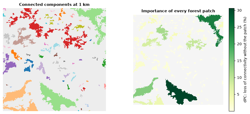
Patches with a high dPCconnector are small but critical: they hold parts of
the network together. node_importance(["IIC", "PC"], ...) computes several
indices at once, and ["BC", "BCIIC", "BCPC"] the betweenness centralities.
Which links matter?
links = forest_net.link_importance("PC", distance=1000, probability=0.5)
links.sort_values("dPC_removal", ascending=False).head()
dPC_removal is the loss of connectivity if a link were cut, e.g. by a new
road. link_change(changes, ...) evaluates new distances for given pairs,
and centrality(distance) returns degree, eigenvector, closeness and
betweenness of every node and its community:
Connectivity of protected areas (ProtConn)
ProtConn is the percentage of a region that is protected and connected. It needs the protected areas and the region as polygons (GeoDataFrames in a metric CRS). As an illustration, treat the large forests of the example as protected areas and the map extent as the region:
import geopandas as gpd
import rasterio.features
import shapely

nodes = ls.conn.node_table(landcover, habitat=[23, 24, 25], area_unit="ha")
patch_area = forest_net.to_raster(nodes, "attribute")
large = (patch_area.values > 200).astype("uint8")                # forests above 200 ha
shapes = rasterio.features.shapes(large, mask=large == 1, transform=landcover.rio.transform())
protected = gpd.GeoDataFrame(geometry=[shapely.geometry.shape(s) for s, _ in shapes],
                             crs=landcover.rio.crs)
region = gpd.GeoDataFrame(geometry=[shapely.box(*landcover.rio.bounds())], crs=landcover.rio.crs)

protconn = ls.conn.protconn(protected, region, distance=[1000, 5000], probability=0.5)
protconn[["distance", "Prot", "ProtConn", "ProtUnconn", "RelConn"]]
Prot is the protected share of the region (%), ProtConn the protected
and connected share, ProtUnconn the difference and RelConn their ratio.
Transboundary protected areas (transboundary=), several regions
(ls.conn.protconn_regions), rasters of protected areas
(ls.conn.protconn_raster) and hexagonal grids (ls.conn.make_grid,
ls.conn.connectivity_grid) are covered in the
API reference.
Networks from habitat patterns
A habitat map analysed with MSPA already contains a network: its cores are
nodes and its bridges links. gtn_components and gtn_importance measure it
directly on the map:
forest = ls.load_raster(ls.example_data("input"))
morph = ls.mspa(forest)
network = ls.gtn_components(morph)
network.num_components, network.eca, network.doc
More
| Task | How |
|---|---|
| Least-cost distances through a resistance map | from_raster(..., distance="least-cost", resistance=resistance) |
| Random-walk (commute-time) distances | distance="commute-time" |
| Connectivity over time, ECA change | ls.conn.eca_change([net_2000, net_2020], "PC", distance=..., landscape_area=...) |
| Candidate patches for restoration | HabitatGraph(..., restoration=flags), then node_importance |
| Connectivity around every patch | ls.conn.focal_nodes(patches, ...) |
| Settlement probabilities of a random walk | HabitatGraph.from_samc(patches, resistance, ...) |
| Export to other software | graph.to_conefor("nodes.txt", "distances.txt") |
Next steps
- Connectivity as current flow across whole landscapes: circuit connectivity.
- Resistance and cost surfaces: distance & restoration.