Chapter 12.10

The planning process¶

Running a solver is a small part of a conservation plan. Most of the work, and most of the value, lies in framing the problem well and in discussing the results with the people who will live with them. This chapter places ls.prioritize in a real planning project, collects good practices and common mistakes, and ends with recipes for common planning questions.

In this chapter

the stages of a systematic conservation plan, and where the software fits;
scenarios rather than "the answer";
good practices and common mistakes;
recipes: 30x30, restoration, offsets, regions, carbon, threats, marine plans, phases;
ls.prioritize for users of prioritizr, prioriactions, Marxan and Zonation.

The stages of a plan¶

Planning projects differ, but most follow a sequence like this (Margules & Pressey 2000; Pressey & Bottrill 2009):

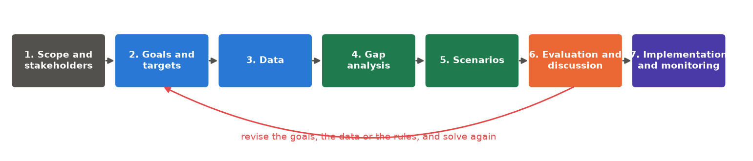
The stages of systematic conservation planning — The stages of a systematic conservation plan. The software works in stages 4 to 6; the loop back from the discussion to the goals is where most plans are made.

Scope and stakeholders. Define the region, the time frame, and who must be involved: agencies, landowners, communities, companies. A technically perfect plan that nobody supports will not be implemented (Knight et al. 2008).
Goals and targets. Turn broad goals ("protect our biodiversity") into measurable targets ("30 % of each ecosystem, 60 % for threatened species").
Data. Gather maps of features, costs, threats, existing protected areas and constraints, on one grid. Chapter 13 makes species maps; chapter 9 costs and distances.
Gap analysis. Measure what existing protected areas already achieve. Some features are often well covered, others not at all.
Scenarios. Solve under different targets, budgets, costs and spatial rules.
Evaluation and discussion. Which places are irreplaceable, which flexible, how do scenarios differ? Show maps and trade-off curves, collect feedback, and return to stage 2 as often as needed.
Implementation and monitoring. Turn the chosen scenario into action (new reserves, restoration contracts, management programmes) and check whether the targets are met on the ground.

Scenarios, not "the answer"¶

A common misunderstanding is to expect one definitive map. Planners produce scenarios that answer "what if" questions:

What if the targets are 20 %, 30 % or 40 %?
What if cost is land price, or the income lost by farmers?
What if existing reserves are, or are not, part of the plan?
What if the plan must be compact, or connected?

Comparing scenarios shows which places are selected whatever the assumptions, strong candidates for immediate action, and which depend on them, open to negotiation. In ls.prioritize scenarios are cheap: every add_ returns a new problem, so one base problem gives many variants (chapter 12.6).

import numpy as np
import pandas as pd
import xarray as xr
import landschaft as ls

P = ls.prioritize
cost = ls.load_raster(P.example_data("cost"))
features = ls.load_raster(P.example_data("features"))
base = P.problem(cost, features).add_min_set_objective().add_binary_decisions()

plans = {t: base.add_relative_targets(t).solve() for t in (0.2, 0.3, 0.4)}
always = np.logical_and.reduce([s.selection.values > 0.5 for s in plans.values()])
print("cells selected in all three scenarios:", int(always.sum()))

Good practices¶

Document every choice. Why this cost layer, these targets, this penalty? A short table of assumptions makes a plan defensible.
Look at the inputs before solving. Most surprising results come from a misaligned raster, a wrong unit or a wrong NoData value. ls.plot(cost) and ls.plot(features) take a second.
Ask for a small gap for final results (add_highs_solver(gap=0.01) or less). The default of 10 % is for exploring, not for reporting.
Calibrate penalties rather than copying values from other studies (chapter 12.6).
Test sensitivity: alternative costs, targets and data, and portfolios of near-optimal plans.
Report target coverage, not only maps: eval_target_coverage_summary says what each scenario achieves for each feature (chapter 12.7).
Share the outputs as GeoTIFFs (sol.save(...) or ls.write_raster(sol.selection, ...)) and as a report (P.report), so that others can inspect them.

Common mistakes¶

Game et al. (2013) list six common mistakes in priority setting. With the pitfalls of the software, they make a useful checklist:

Treating the map as a decision

The map shows the consequences of the chosen inputs. It is a starting point for negotiation.

Ignoring costs, or mixing their units

Plans without costs favour expensive places; costs in different currencies or time frames (a purchase price plus a yearly management cost) make meaningless plans. Put all costs in one currency and one time frame.

Confusing threat with priority

The most threatened place is not always the best investment: action there may be expensive, or unlikely to work. Multi-action planning (chapter 12.8) weighs both.

Forgetting that the cost raster defines the planning units

A zero is a planning unit that costs nothing, and the solver will take it; NoData is not a planning unit at all.

Too many features of one kind

With 500 bird species and one ecosystem type, birds drive the plan. Group features, weight them, or set targets per group.

Ignoring the probability of success, and what would happen anyway

Protecting land nobody would ever clear adds little. Where it is known, weight benefit by the threat that action removes, and cost by the chance of success.

Recipes¶

The same few building blocks answer very different questions. Each recipe gives the question, how it translates into a problem, and code on Serra Verde that you can adapt to your own data.

National 30x30 strategy¶

"Which new areas complete our network so that 30 % of every ecosystem is protected?" A gap analysis, then a minimum set that builds on the existing reserves and excludes land that is not available:

protected = ls.load_raster(P.example_data("protected"))
urban = ls.load_raster(P.example_data("urban"))
p = base.add_relative_targets(0.3)

gap = P.eval_target_coverage_summary(p, protected)        # what the reserves hold today
print(gap[["feature", "relative_held"]].round(2).to_string(index=False))

plan = p.add_locked_in_constraints(protected).add_locked_out_constraints(urban).solve()
new = (plan.selection.values > 0.5) & (np.nan_to_num(protected.values) == 0)
print(f"new areas: {int(new.sum())} km², {np.nansum(cost.values * new) / 1000:.1f} million USD")

Restoration¶

"Where should we restore degraded land to recover the most biodiversity per dollar?" The benefit of restoring is the gain, not the habitat present today. Here the gain of a cell is its habitat times its degradation, and any share of a cell can be restored:

condition = ls.load_raster(P.example_data("condition"))
gain = features * (1 - condition)                           # habitat that restoration would bring back
restore = (P.problem(cost, gain).add_max_utility_objective(5_000)
             .add_proportion_decisions().solve())
print(f"cells restored at least in part: {int((restore.values > 0.01).sum())}")

Use gains, not current habitat

With today's habitat as features, the plan "restores" the places already in good condition. Estimate the gain first: from condition, as here, or from distribution models under the restored land cover.

Biodiversity offsets¶

"Where should a company compensate the habitat lost to a new road?" Absolute targets equal to the losses (times an offset ratio), outside the footprint and the existing reserves (additionality):

footprint = xr.zeros_like(cost).where(np.isfinite(cost))
footprint[40:46, 30:42] = 1                                   # the project's area
lost = (features * footprint).sum(["y", "x"]).values         # habitat lost, per feature
eligible = cost.where((footprint == 0) & (np.nan_to_num(protected) == 0))
offset = (P.problem(eligible, features).add_min_set_objective()
            .add_absolute_targets(2 * lost).add_binary_decisions().solve())   # an offset ratio of 2
print(f"offset: {int(offset.values.sum())} km², {offset.cost / 1000:.1f} million USD")

Plans across regions¶

"How do we share the effort fairly between three states?" A plan for the whole region concentrates the effort where land is cheapest. Subregional targets require 30 % of each feature within each state. The difference in cost is the price of fairness:

regions = ls.load_raster(P.example_data("regions"))          # 1, 2, 3
names = [str(n) for n in features.band.values]
targets = pd.DataFrame([{"region": r, "feature": f, "target": 0.3} for r in (1, 2, 3) for f in names])
fair = base.add_relative_targets(0.0).add_subregional_targets(regions, targets).solve()
whole = base.add_relative_targets(0.3).solve()
print(f"price of fairness: {fair.cost / whole.cost - 1:.1%}")

A feature absent from a state gets a target of zero there. Compare also the share of each state's land the two plans select.

Carbon as a co-benefit¶

"Can the plan also store carbon?" Add carbon as a feature. With a target of zero it is only measured; with a target, it is required:

carbon = ls.load_raster(P.example_data("carbon"))
with_carbon = xr.concat([features, carbon.expand_dims(band=["carbon"])], dim="band")
pc = P.problem(cost, with_carbon).add_min_set_objective().add_binary_decisions()
species_only = pc.add_relative_targets([0.3] * 8 + [0.0]).solve()
held = P.eval_feature_representation_summary(pc.add_relative_targets(0.3), species_only)["relative_held"]
print(f"the species plan holds {held.iloc[-1]:.0%} of the carbon")
for t in (0.25, 0.3):
    s = pc.add_relative_targets([0.3] * 8 + [t]).solve()
    print(f"{t:.0%} of the carbon: {s.cost / species_only.cost - 1:.0%} dearer")

The plan for the species already holds a fifth of Serra Verde's carbon. A quarter costs about 8 % more, and 30 % costs 28 % more: carbon is everywhere, so every extra share of it means much more land. Curves like this one (chapter 12.6) help to set carbon targets that are ambitious but affordable.

Threat management¶

"Which threats should we tackle, and where?" A multi-action plan with threats, actions and their costs: see chapter 12.8.

Marine plans¶

"Where can no-take zones go while displacing as little fishing as possible?" A minimum set with fishing effort as the cost, shipping lanes locked out, and a boundary penalty with edge_factor=1, since zones must be simple to enforce:

effort = ls.load_raster("fishing_effort.tif")             # the cost: fishing displaced
habitats = ls.load_raster("habitats.tif")                 # reefs, seagrass, spawning areas
plan = (P.problem(effort, habitats).add_min_set_objective().add_relative_targets(0.2)
          .add_binary_decisions().add_locked_out_constraints(ls.load_raster("shipping_lanes.tif"))
          .add_boundary_penalties(calibrated_value, edge_factor=1.0)
          .solve())

Report the share of fishing effort displaced, not only the area protected.

Plans in phases, and extinction risk¶

"We can only act on part of the plan each year: where do we start?" Rank the plan's units by importance (chapter 12.7) or build it in phases with iterative_solve (chapter 12.6). "Which areas reduce extinction risk the most?" The minimum extinction risk objective (chapter 12.4).

Coming from R or Marxan¶

ls.prioritize follows the vocabulary of prioritizr, so most scripts translate line by line:

prioritizr (R)	`ls.prioritize`
`problem(cost, features)`	`P.problem(cost, features)`
`add_min_set_objective()` and the others	the same names, as methods: `p.add_min_set_objective()`
`add_relative_targets(0.3)`	`p.add_relative_targets(0.3)`
`add_boundary_penalties(penalty, edge_factor)`	`p.add_boundary_penalties(penalty, edge_factor)`
`add_locked_in_constraints(x)`	`p.add_locked_in_constraints(x)`
`add_binary_decisions()`	`p.add_binary_decisions()`
`add_highs_solver(gap = 0.1)`	`p.add_highs_solver(gap=0.1)`
`solve(p)`	`p.solve()`
`eval_target_coverage_summary(p, s)`	`P.eval_target_coverage_summary(p, s)`
`compile(p)`	`p.compile()` (the same model, row by row)

Pipes (%>%) become method chains, and every method returns a new problem. Extensions beyond prioritizr: subregional targets, corridors, minimum extinction risk, calibration helpers, and the comparison with Zonation.

Other tools	In `ls.prioritize`
prioriactions (`inputData`, `problem`, `solve`)	`actions_data`, `ActionsData.problem`, `ActionsProblem.solve`
Marxan (`input.dat`, `pu.dat`, `spec.dat`, `puvspr.dat`)	`P.marxan(pu, spec, puvspr, bound, blm=...)`, the same tables
Zonation 5 (`z5 --mode=CAZ2 settings.z5`)	`P.zonation(...)`, or `P.run_project("settings.z5")`

Results are the same as the originals': prioritizr and prioriactions models agree row by row, Marxan with the same seed gives the same runs, and Zonation 5 the same ranking. That makes it easy to move an existing analysis and check it. The migration guide has the full dictionary, function by function, for prioritizr, prioriactions and prioripy.

Key points

The software works in the middle of a longer process; goals, data and discussion matter more.
Produce scenarios; trust the places selected in all of them.
Document choices, check inputs, use small gaps for final plans, calibrate penalties, report coverage.
Most planning questions are recipes of the same ingredients: targets, costs, locks, objectives.

Check your understanding¶

A stakeholder asks why their land is in the plan. What would you show them?
Why lock out existing reserves in an offset problem?
In Serra Verde, the price of fairness between the three states is 9 %. Is that a lot?

Answers

Its importance (replacement cost or irreplaceability), the features it holds that are rare elsewhere, and whether near-optimal alternatives without it exist (a portfolio). If there are, the plan can do without it at a small cost.
Additionality: protecting land already protected does not compensate any loss.
It depends on the budget and the stakes, but it is often a small price for a plan every state can accept. A plan that is 9 % cheaper but rejected by two states protects nothing.

References¶

Game, E. T., Kareiva, P., & Possingham, H. P. (2013). Six common mistakes in conservation priority setting. Conservation Biology, 27(3), 480–485.
Hanson, J. O., Schuster, R., Strimas-Mackey, M., Morrell, N., Edwards, B. P. M., Arcese, P., Bennett, J. R., & Possingham, H. P. (2025). Systematic conservation prioritization with the prioritizr R package. Conservation Biology, 39(1), e14376.
Knight, A. T., Cowling, R. M., Rouget, M., Balmford, A., Lombard, A. T., & Campbell, B. M. (2008). Knowing but not doing: selecting priority conservation areas and the research–implementation gap. Conservation Biology, 22(3), 610–617.
Kukkala, A. S., & Moilanen, A. (2013). Core concepts of spatial prioritisation in systematic conservation planning. Biological Reviews, 88(2), 443–464.
Margules, C. R., & Pressey, R. L. (2000). Systematic conservation planning. Nature, 405, 243–253.
Pressey, R. L., & Bottrill, M. C. (2009). Approaches to landscape- and seascape-scale conservation planning: convergence, contrasts and challenges. Oryx, 43(4), 464–475.
Strassburg, B. B. N., Iribarrem, A., Beyer, H. L., Cordeiro, C. L., Crouzeilles, R., Jakovac, C. C., et al. (2020). Global priority areas for ecosystem restoration. Nature, 586, 724–729.