Optimized conservation plans

Which set of places meets a conservation goal at the least cost, or achieves the most with a fixed budget? ls.prioritize answers it with exact optimization, as the R package prioritizr does (the same models, row by row), with engines of its own that solve large and spatial problems much faster. This tutorial builds a complete plan for Serra Verde, the example region of the course chapters 12.1 to 12.10, which explain the ideas behind every step.

You will learn to:

• set up a problem from cost and feature rasters, and run a gap analysis of existing reserves;
• solve a minimum-set plan that builds on the reserves and avoids the cities;
• make it compact with a calibrated boundary penalty;
• see what each budget buys;
• find the places that matter most, and the alternatives;
• plan actions against threats;
• give every unit a zone: protection, sustainable use or restoration;
• compare with a Zonation ranking, and share the results.

The data

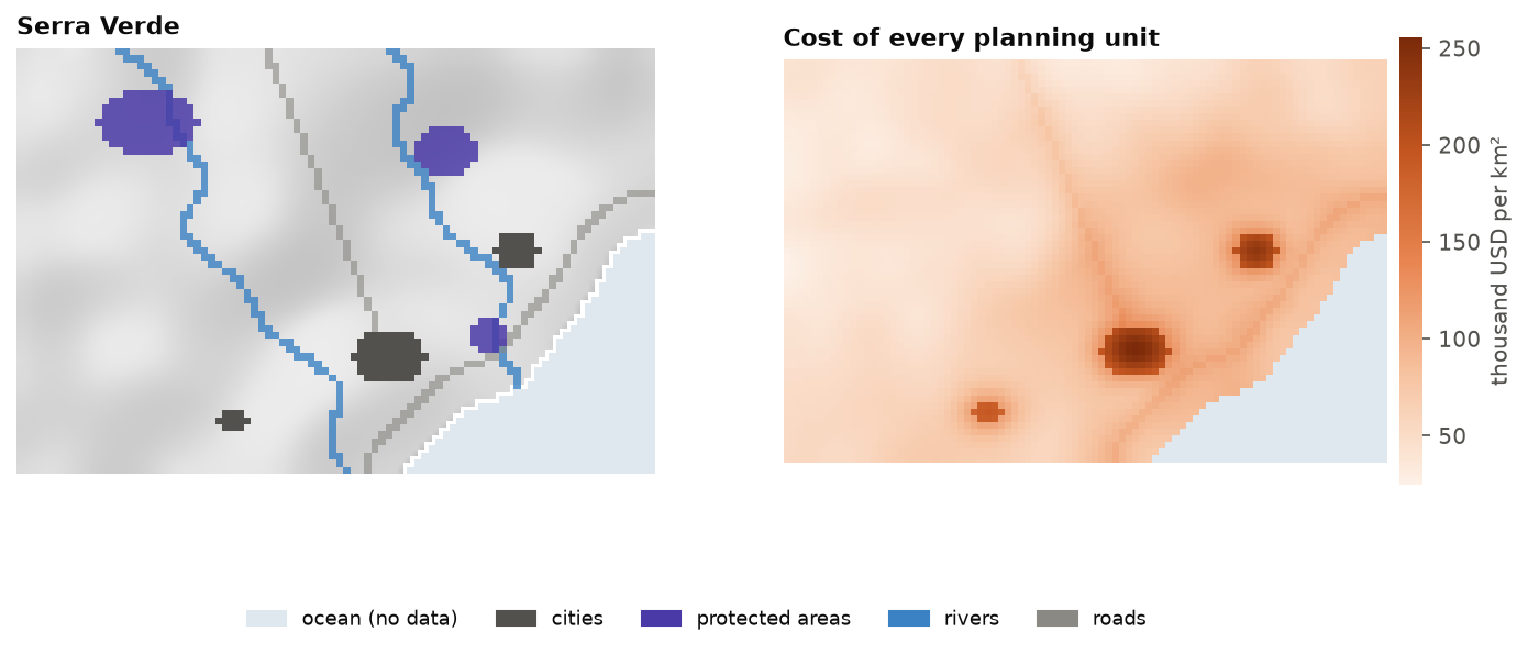
Serra Verde ships with Landschaft: 60 x 90 cells of 1 km, with a land cost, eight features, three protected areas, three cities and two threats. The cost raster defines the planning units: its 4825 cells with a value.

import numpy as np
import pandas as pd
import landschaft as ls

P = ls.prioritize
cost = ls.load_raster(P.example_data("cost"))            # thousand USD per km²
features = ls.load_raster(P.example_data("features"))    # habitat suitability, 8 bands
protected = ls.load_raster(P.example_data("protected"))  # existing reserves (1)
urban = ls.load_raster(P.example_data("urban"))          # cities (1)
[str(b) for b in features.band.values]

What the reserves hold today

A problem combines planning units, features, an objective, targets and decisions. Before solving it, evaluate the existing reserves as if they were a plan, a gap analysis:

p = (P.problem(cost, features)
       .add_min_set_objective()
       .add_relative_targets(0.3)
       .add_binary_decisions())

P.eval_target_coverage_summary(p, protected)[["feature", "relative_held", "met"]].round(3)

The three reserves hold up to a tenth of the mountain species and nothing of the tapir, the tamarin and the mangrove. None of the targets of 30 % is met.

A first plan

The cheapest set of cells that meets every target, keeping the reserves and leaving out the cities:

p1 = (p.add_locked_in_constraints(protected)
        .add_locked_out_constraints(urban)
        .add_highs_solver(gap=0.001))
plan = p1.solve()
print(plan.status, f"cost {plan.cost / 1000:.1f} million USD, {int(plan.values.sum())} cells, gap {plan.gap:.3%}")
plan.coverage[["feature", "relative_target", "relative_held", "met"]].round(3)

plan.selection is the plan as a raster, ls.plot(plan) draws it, and plan.save("plan.tif") writes it. The solver proves the plan is within 0.1 % of the cheapest possible (the gap, chapter 12.4).

A compact plan

The plan is scattered over many patches. A boundary penalty makes it compact at some extra cost. Its value must be calibrated: solve with several values and choose on the curve of cost against boundary (chapter 12.6):

cal = P.calibrate_penalty(p1.add_highs_solver(gap=0.02), "boundary", values=[0.001, 0.003, 0.01, 0.03])
cal.table[["value", "cost", "boundary", "knee", "topsis"]].round(1)

compact = cal.best("knee")
for name, s in (("first plan", plan), ("compact plan", compact)):
    lm = P.eval_landscape_metrics(s, metric="np")
    km = P.eval_boundary_summary(p1, s)["boundary"].iloc[0] / 1000
    print(f"{name:13s} {s.cost / 1000:5.1f} million USD, {km:4.0f} km of boundary, "
          f"{int(lm['value'].iloc[0])} patches")

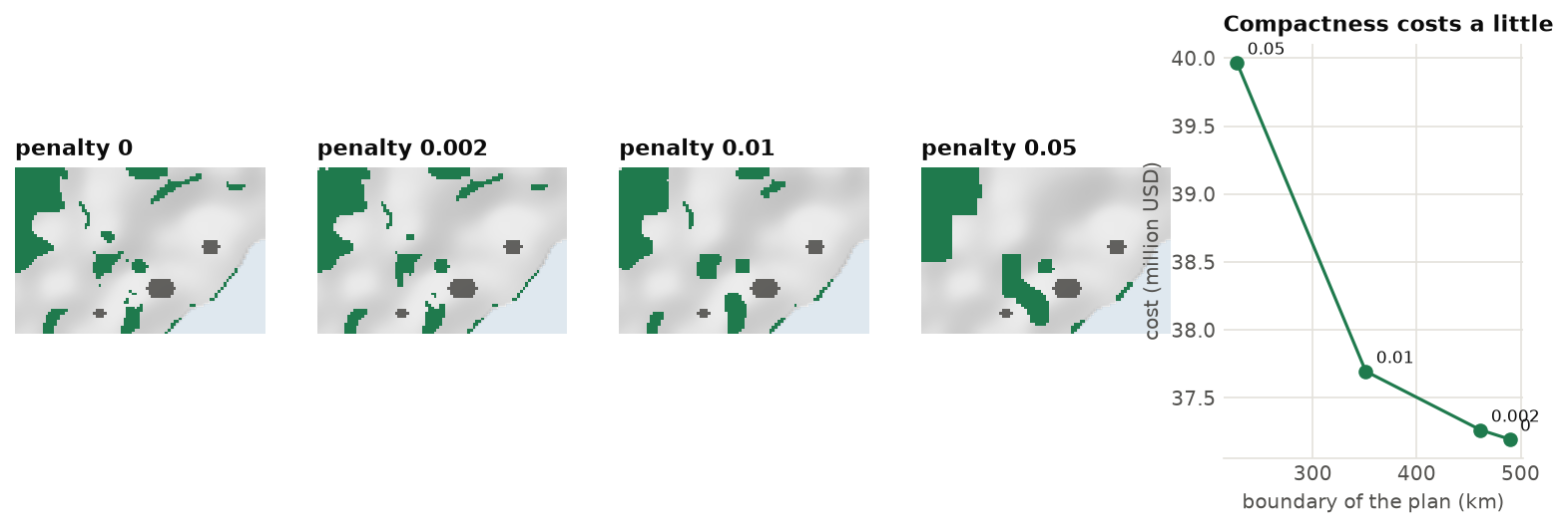
The knee of the curve buys a much shorter boundary, in fewer patches, for a small part of the cost. ls.plot(cal) draws the curve.

What each budget buys

Decision makers often ask what a budget buys rather than what a target costs. The Pareto front solves the minimum shortfall problem for a range of budgets:

front = P.pareto_front(p1, n=6)
front.table[["value", "shortfall", "met"]].round(2)

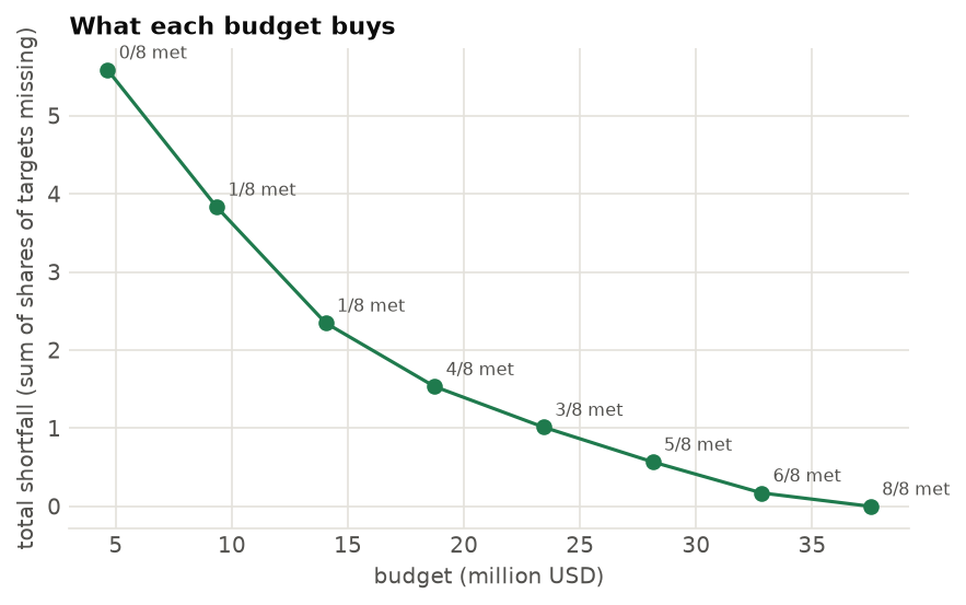
The shortfall (the share of the targets still missing, summed over the features) falls fast with the first millions and slowly with the last. Every budget includes the reserves, so the front starts above their cost. (The figure shows the front of the plan without reserves.)

The places that matter most

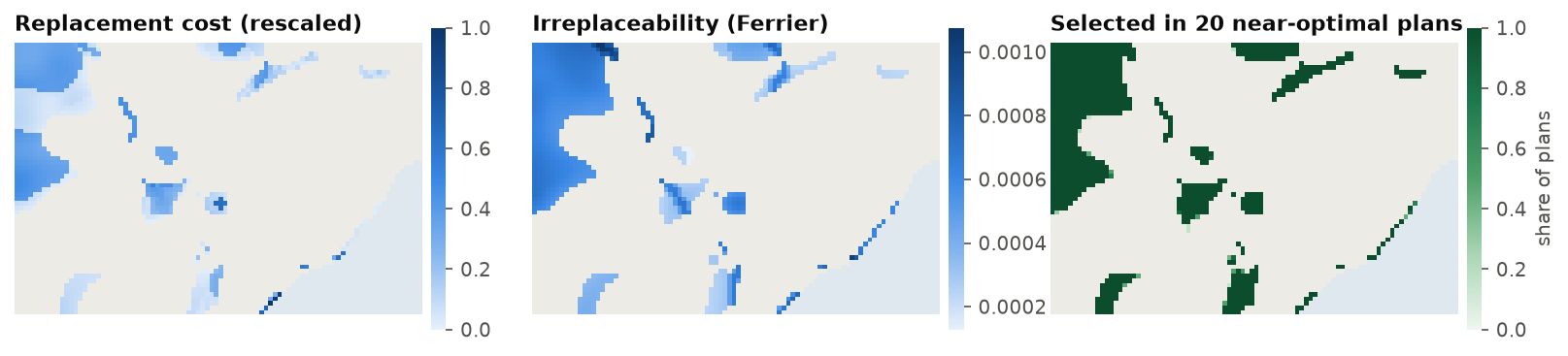
Which cells could not be replaced? Replacement cost solves the problem again without each selected cell; a portfolio of near-optimal plans shows which cells are always chosen (chapter 12.7):

rc = P.eval_replacement_importance(p1, plan)
port = p1.add_highs_solver(gap=0.01).add_gap_portfolio(10, pool_gap=0.02).solve()
f = port.frequency.values
print(f"{len(port)} plans within 2 %: {int(np.nansum(f == 1))} cells in all of them, "
      f"{int(np.nansum((f > 0) & (f < 1)))} in some")

Actions against threats

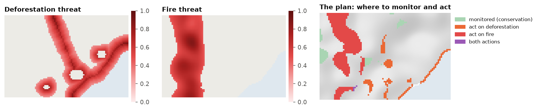
Deforestation and fire threaten the features. A multi-action plan decides where to manage land and where to act against each threat (chapter 12.8):

threats = ls.load_raster(P.example_data("threats"))
d = P.actions_raster_data(cost, features, threats, action_cost=[30, 10],
                          target_recovery=0.3, target_conservation=0.1)
acts = d.problem("minimizeCosts").add_highs_solver(gap=0.01).solve()
print(f"{int(acts.units.sum())} cells managed, {int(acts.actions.sum())} actions")
acts.cost()

Zones of management

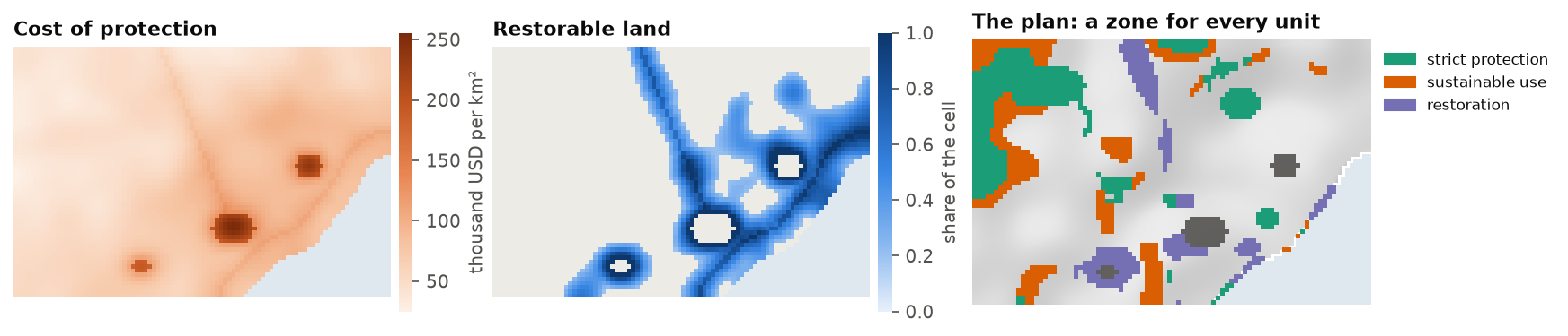
A plan can also give every unit a zone: strict protection, sustainable use or restoration, each with its own cost and its own worth for the features. Sustainable use is cheaper but counts half of every feature; restoring pasture and cropland brings back their share of the cell; the targets are met by the sum over the zones, and 10 % of every feature must be under strict protection (chapter 12.8):

lc = ls.load_raster(P.example_data("land_cover"))
anthropic = lc.sel(band="pasture") + lc.sel(band="cropland")      # restorable share of every cell
costs = {"protect": cost,
         "use": cost * 0.45,
         "restore": (cost * 0.2).where(anthropic > 0.2)}         # no cost: the unit cannot go there
pz = (P.problem(costs, features, contribution={"use": 0.5, "restore": anthropic})
        .add_min_set_objective()
        .add_relative_targets(0.3)                    # 30 % of every feature, counted in every zone
        .add_relative_targets(0.1, zone="protect")    # and 10 % of it strictly protected
        .add_locked_in_constraints({"protect": protected})
        .add_locked_out_constraints({z: urban for z in costs})
        .add_boundary_penalties(0.0005)               # compact zones
        .add_highs_solver(gap=0.02))
zplan = pz.solve()
{z: round(c) for z, c in zplan.zone_costs.items()}

The plan keeps the reserves under protection, puts 560 cells under strict protection, 450 under sustainable use and restores 284, for 40 450 thousand USD. zplan.zones is the map of the zones, and every evaluation gives a row overall and one per zone:

P.eval_n_summary(pz, zplan)

Compared with a Zonation ranking

A Zonation ranking cut at the same cost holds more of the rare features and less of the common ones (chapter 12.9):

comp = P.compare_zonation(p1, plan)
comp.table[["feature", "milp", "zonation"]].round(2)

Sharing the results

report gathers the summaries, representation, targets and importance; ls.plot makes a web page of them:

r = P.report(p1, plan, extinction_z=0.25)
page = ls.plot(r, show=False).save("serra_verde_plan.html")

Going further

• Other objectives: maximum utility, minimum shortfall, maximum features, phylogenetic diversity, and minimum extinction risk (chapter 12.4).
• Spatial rules: neighbours, contiguity, corridors and connectivity (chapter 12.5).
• Polygons and H3 cells as planning units: P.problem(polygons, features, cost_column="cost"), P.h3_units(cost, resolution).
• Large problems: coarsen and refine (chapter 12.9).
• Marxan: P.marxan runs Marxan's own tables and annealing; add_anneal_solver solves a problem with it.
• Restoration: how much of every converted cell to restore, for species, carbon and intactness: restoration priorities.
• Recipes for 30x30, restoration, offsets, regions and carbon: chapter 12.10.
• The API reference lists every function.