Chapter 2

Scale

Ask how fragmented a forest is and the honest answer begins with "at what scale?". Seen through 10 m pixels, a forest crossed by tracks and clearings is a mosaic of pieces; through 1 km pixels it is a single block. Seen around a single tree it is intact; over a whole region it may be rare. Levin (1992) called scale the central problem in ecology: there is no single correct scale at which to describe a system, and every measurement of pattern is made at some scale, chosen or not.

In this chapter

• the components of scale: grain, extent and thematic resolution;
• how landscape measurements change with each of them, shown on the example maps;
• the scale of effect: the extent at which a landscape matters to an organism;
• how scale enters every tool of Landschaft, and practical rules for choosing it.

The components of scale

In landscape ecology, scale has precise components (Turner et al., 1989; Wiens, 1989):

Component	Definition	In a raster map
Grain	the finest level of spatial resolution	the cell size (25 m, 30 m, 1 km...)
Extent	the overall size of the area studied	the size of the map, plot or window
Thematic resolution	how finely the categories are defined	the number of classes of the legend
Temporal grain and extent	how often, and over how long, the landscape is observed	the dates of the maps

Grain and extent bound what can be seen. Nothing smaller than the grain can be detected, and nothing larger than the extent. A 30 m land-cover map cannot show hedgerows 5 m wide; a map of one municipality cannot show a migration route of 200 km.

Two other notions of scale must not be confused with these:

• The cartographic scale of a paper map (1:25 000) is a ratio; a "large" cartographic scale shows a small area in detail. Ecologists say "large scale" to mean a large extent. Avoid the ambiguity: speak of grain and extent.
• The minimum mapping unit (MMU) is the smallest area a map delineates. It can be much larger than the cell size: the CORINE map used in this course has 25 m cells but was drawn with an MMU of 25 ha. Its effective grain is therefore about 500 m, not 25 m.

Grain: the same landscape at different resolutions

Most landscape measurements change with the grain, some predictably and some erratically (Turner et al., 1989; Wu, 2004). Let us see it happen. We take the binary forest map of the examples and make it coarser by majority rule: each block of k × k cells becomes one cell, forest if at least half of the block is forest.

import numpy as np
import landschaft as ls

forest = ls.load_raster(ls.example_data("input")).values   # 0 missing, 1 background, 2 forest


def coarsen(habitat, k):
    """Majority aggregation of k x k blocks of a 0/1/2 habitat map."""
    n_rows, n_cols = habitat.shape[0] // k, habitat.shape[1] // k
    blocks = habitat[: n_rows * k, : n_cols * k].reshape(n_rows, k, n_cols, k)
    share = (blocks == 2).mean(axis=(1, 3))
    return np.where(share >= 0.5, 2, 1).astype("uint8")

We treat the cells of this map as 25 m, as the tutorials do, and compute four class metrics of the forest at grains from 25 to 400 m:

import pandas as pd

rows = []
for k in [1, 2, 4, 8, 16]:
    grain = 25 * k                                           # metres
    metrics = ls.Landscape(coarsen(forest, k), res=grain).class_metrics(
        ["pland", "np", "area_mn", "ed"])
    rows.append(metrics[metrics["class"] == 2].assign(grain_m=grain))

by_grain = pd.concat(rows).set_index("grain_m")[["pland", "np", "area_mn", "ed"]]
by_grain.round(1)

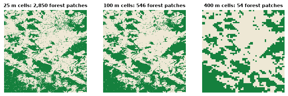
Read the table column by column:

• Percentage of forest (pland) barely moves, 40–46%: majority aggregation roughly preserves the amount of each class. Composition is fairly robust to grain.
• Number of patches (np) falls from about 2 850 to about 50: small patches disappear, and patches separated by narrow gaps merge.
• Mean patch area (area_mn) grows about fifty-fold, the mirror image of the number of patches.
• Edge density (ed) falls about six-fold: coarse cells smooth the boundaries, and edges shorter than a cell vanish.

Configuration metrics, those that describe the arrangement of patches, are the most sensitive. This is why a statement such as "the forest has 2 850 patches" means nothing without its grain, and why landscapes can only be compared at the same grain (Wu, 2004).

Majority rule is only one way to aggregate

Coarsening by majority removes minority classes from every block, so rare and linear features (hedges, rivers, roads) disappear first. Other rules (random, nearest, "any presence") give different results. When you must compare maps of different resolutions, resample them all to the coarsest grain with the same rule, and report it.

Thematic resolution

The number of classes matters as much as the cell size (Buyantuyev & Wu, 2007). CORINE Land Cover has three nested levels: 44 classes, grouped in 15, grouped in 5. Merging the 26 classes present in the example into the five top-level groups (artificial, agricultural, forest and semi-natural, wetlands, water):

landcover = ls.load_raster(ls.example_data("clc"))
level1 = ls.reclassify(landcover, [(1, 12, 1),     # artificial surfaces
                                   (12, 23, 2),    # agricultural areas
                                   (23, 35, 3),    # forest and semi-natural areas
                                   (35, 40, 4),    # wetlands
                                   (40, 45, 5)])   # water

compare = pd.concat({
    "26 classes": ls.Landscape(landcover).landscape_metrics(["pr", "np", "shdi", "ed"]),
    "5 classes": ls.Landscape(level1).landscape_metrics(["pr", "np", "shdi", "ed"]),
})
compare.round(2)

The landscape did not change; the legend did. Yet the number of patches halves, the Shannon diversity (shdi, chapter 5) falls from 1.8 to 1.0 and the edge density by a third, because boundaries between classes of the same group are no longer edges. Diversity and edge metrics depend on the legend by construction. Choose the classes for the question (a forest bird does not distinguish broad-leaved from mixed forest if both serve it) and keep them fixed across the landscapes you compare.

Extent

Enlarging the extent adds new patches and classes and, eventually, new kinds of landscape. Two effects are worth remembering:

• The map border truncates patches. Patches cut by the edge of the map look smaller and have artificially straight boundaries. The smaller the extent relative to the patches, the stronger the bias. Landschaft follows the convention of FRAGSTATS and landscapemetrics: the map border is not counted as edge unless you ask (count_boundary=True).
• Rare classes need large extents. Class-level metrics of a class with three patches in the study area are dominated by chance.

O'Neill et al. (1996) proposed a rule of thumb that is still useful: the grain should be two to five times smaller than the smallest features of interest, and the extent two to five times larger than the largest patches.

The scale of effect

For an organism, which part of the landscape matters? A population of forest birds in a woodlot responds to the forest around it, but within what radius: 250 m, 1 km, 5 km? The extent at which landscape structure best predicts a biological response is the scale of effect (Jackson & Fahrig, 2012). It depends on the species (dispersal distance, home range), on the response (abundance, occupancy, genetic diversity) and on the landscape variable itself (Holland et al., 2004; Miguet et al., 2016).

The standard way to find it is a multi-scale analysis: measure the landscape in buffers of several radii around each sampling site, relate each radius to the response, and keep the radius with the strongest relation. Studies that choose one radius a priori, without testing, often miss the scale of effect and underestimate the effect of the landscape (Jackson & Fahrig, 2015).

Landschaft computes the landscape side of such an analysis in one call. Here are three hypothetical sites, and the percentage of forest within circles of 250 m to 4 km around each:

xmin, xmax, ymin, ymax = ls.Landscape(landcover).extent
sites = np.array([[xmin + 12_000, ymin + 12_000],
                  [xmin + 25_000, ymin + 25_000],
                  [xmax - 12_000, ymax - 12_000]])
radii = [250.0, 500.0, 1000.0, 2000.0, 4000.0]

forest_lc = ls.reclassify(landcover, foreground=[23, 24, 25])
plots = ls.scale_sample(forest_lc, sites, size=radii, shape="circle",
                        what=["lsm_c_pland"], verbose=False)

forest_share = (plots[plots["class"] == 2]
                .pivot(index="plot_id", columns="size", values="value")
                .reindex(index=[1, 2, 3], columns=radii)
                .fillna(0.0))                 # no forest in the circle: 0%
forest_share.round(1)

All three sites lie in open farmland (0% forest within 500 m) but in landscapes with 9 to 24% forest within 4 km. Whether site 2 is "less forested" than site 3 depends on the radius: at 2 km they are close, at 4 km site 3 has three times more forest. With a response variable measured at each site (say, the abundance of a forest bird), you would correlate it with each column and keep the radius that explains it best.

Scale in the tools of Landschaft

Almost every tool has a scale parameter. Most are counted in cells, so their meaning on the ground depends on the grain:

Parameter	Tools	Sets	On the ground
window_size	density, fragmentation, mosaic, window metrics	the neighbourhood of every cell	side = cells × grain
edge_width	MSPA, SPA	how deep edge effects reach	depth = cells × grain
edge_depth	core-area metrics	the same, for patch metrics	depth = cells × grain
size	sample plots, scale_sample	the radius (circle) or half-side (square)	map units
distance, max_distance	habitat networks	dispersal distance	map units
radius	omnidirectional circuits	the reach of movement	cells × grain

A 27-cell window over 25 m cells covers 675 m × 675 m, about 46 ha; over 30 m Landsat cells it covers 810 m × 810 m, about 66 ha. When you move an analysis to a map of another resolution, convert the parameters so that the distances on the ground stay the same, and report them in metres, not in cells.

Choosing scales in practice

1. Start from the biology: dispersal distance, home range, the depth of edge effects, the size of the management unit.
2. Check that the map can resolve it (grain) and contains it (extent).
3. When the right scale is unknown, analyse several and report them all: fad_multiscale does this for habitat density, scale_sample for metrics around points, and the network tools accept lists of distances.
4. Report grain, extent, legend and every scale parameter in map units.

Key points

• Scale has components: grain, extent and thematic resolution. Each changes the values of landscape measurements.
• Composition (how much of each class) is more robust to grain than configuration (how it is arranged).
• A map's effective grain can be coarser than its cell size (the minimum mapping unit).
• The scale of effect is found empirically by multi-scale analysis.
• Compare landscapes only at the same grain, extent and legend, and report scale parameters in map units.

Check your understanding

1. A study reports that a forest reserve "has an edge density of 45 m/ha". What else do you need to know to compare it with another reserve?
2. You run an analysis with window_size=27 on a 10 m map, then on a 100 m map of the same area. Are the two results comparable? What would make them so?
3. Why might two studies of the same bird species report different scales of effect?

Answers

1. The grain and the minimum mapping unit of the map, its legend (what counts as edge), whether the map border was counted as edge, and the extent.
2. No: the windows cover 270 m and 2.7 km on the ground. Use a window of about 27 × 10 / 100 ≈ 3 cells on the 100 m map (the nearest odd size), and remember that the coarser map has also lost the finest features.
3. Because the scale of effect depends on the response variable (abundance, occupancy, breeding success), on the landscape variable, on the region (landscapes with different structure) and on the range of radii tested; it is not a fixed property of the species.

References

• Buyantuyev, A., & Wu, J. (2007). Effects of thematic resolution on landscape pattern analysis. Landscape Ecology, 22, 7–13.
• Holland, J. D., Bert, D. G., & Fahrig, L. (2004). Determining the spatial scale of species' response to habitat. BioScience, 54(3), 227–233.
• Jackson, H. B., & Fahrig, L. (2012). What size is a biologically relevant landscape? Landscape Ecology, 27, 929–941.
• Jackson, H. B., & Fahrig, L. (2015). Are ecologists conducting research at the optimal scale? Global Ecology and Biogeography, 24(1), 52–63.
• Levin, S. A. (1992). The problem of pattern and scale in ecology. Ecology, 73(6), 1943–1967.
• Miguet, P., Jackson, H. B., Jackson, N. D., Martin, A. E., & Fahrig, L. (2016). What determines the spatial extent of landscape effects on species? Landscape Ecology, 31, 1177–1194.
• O'Neill, R. V., Hunsaker, C. T., Timmins, S. P., Jackson, B. L., Jones, K. B., Riitters, K. H., & Wickham, J. D. (1996). Scale problems in reporting landscape pattern at the regional scale. Landscape Ecology, 11, 169–180.
• Turner, M. G., O'Neill, R. V., Gardner, R. H., & Milne, B. T. (1989). Effects of changing spatial scale on the analysis of landscape pattern. Landscape Ecology, 3, 153–162.
• Wiens, J. A. (1989). Spatial scaling in ecology. Functional Ecology, 3(4), 385–397.
• Wu, J. (2004). Effects of changing scale on landscape pattern analysis: scaling relations. Landscape Ecology, 19, 125–138.