Surface texture¶

Not every landscape is a mosaic of patches. Vegetation greenness, canopy height, soil moisture, elevation vary continuously, and classifying them into habitat and non-habitat throws most of that variation away. Surface metrics describe a continuous raster as it is: how much it varies, how its heights are distributed, how steep and rough it is, whether its texture has a direction or a dominant wavelength. They come from the ISO 25178 standard for engineered surfaces, brought to landscape ecology as gradient surface metrics (McGarigal et al. 2009).

You will learn to:

remove a trend from a surface and describe what remains with amplitude, slope and feature metrics;
read the bearing area curve of a surface and its parameters;
map texture with metrics in a moving window;
measure the spatial structure of a surface: correlation lengths, texture direction and wavelength, fractal dimension;
compute terrain indices of a DEM: slope, TPI, ruggedness, curvature, heat load;
classify landforms with geomorphons;
delineate the hilltops protected by Brazil's Forest Code.

Everything lives in ls.surface. The metrics follow the R packages geodiv (surface metrics) and spatialEco (terrain indices), value for value where they are right; where they err, each function's notes say what is corrected.

A surface and its trend¶

The example data are three rasters of about 30 m cells over south-western Oregon: summer NDVI, the same NDVI with its trend removed, and elevation. Surface metrics describe variation around a reference plane, so a broad trend (a gradient of greenness across the map) is removed first.

import landschaft as ls

ndvi = ls.load_raster(ls.surface.example_data("orforest"))
z = ls.surface.remove_plane(ndvi)
print(z.attrs["order"], round(float(z.mean()), 12))

2 0.0

remove_plane fits least-squares polynomial surfaces of order 0 to 3 in the cell coordinates and subtracts the one with the least BIC; fit_plane gives a surface of a chosen order. What remains, the residual surface, is what the metrics describe.

Whole-surface metrics¶

ls.surface.metrics computes every metric at once (or those named), and metrics that share a computation are computed once:

m = ls.surface.metrics(z, ["sa", "sq", "ssk", "sku", "sdq", "sds", "s10z", "sdr"])
print(m.round(4))

sa      0.0437
sq      0.0643
ssk    -1.9820
sku     6.8255
sdq     0.0439
sds     0.0480
s10z    0.6661
sdr     0.1773
dtype: float64

Amplitude. Sa is the mean absolute deviation from the mean height, Sq the root mean square. Ssk and Sku describe the height distribution: a negative skewness means deep valleys among a high plateau (here: patches of low greenness in a green forest), a large kurtosis a peaked distribution with long tails.
Slopes. Sdq is the root mean square slope (height change per cell), Sdr how much larger the surface is than its footprint, in percent.
Features. Sds counts peaks (cells higher than their 8 neighbours) per cell; S10z averages the five highest peaks and five deepest valleys.

ls.surface.list_metrics() lists all 27.

The bearing area curve¶

The bearing area (Abbott-Firestone) curve sorts the heights: for every height, the share of the surface at or above it. Its shape tells where the material is. A core line fitted through the flattest 40 % of the curve separates the peaks above it (Spk), the core (Sk) and the valleys below (Svk); Sbi compares Sq with the height at 5 % bearing, Sci and Svi measure the void volume of the core and valley zones.

curve = ls.surface.bearing_area(z)
print(ls.surface.height_ba(z, [0, 0.05, 0.5, 0.95, 1]).round(4))
print(ls.surface.metrics(z, ["sbi", "sci", "svi", "sk", "spk", "svk"]).round(4).to_dict())

[ 0.1485  0.0798  0.0105 -0.1144 -0.5872]
{'sbi': 0.8063, 'sci': 0.0679, 'svi': 0.0127, 'sk': 0.1041, 'spk': 0.0863, 'svk': 0.5453}

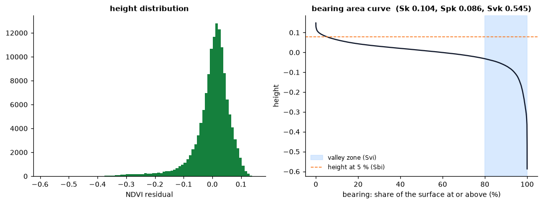
Height distribution and bearing area curve of the NDVI residuals

The deep tail of low-greenness cells shows as a long valley zone: Svk is several times Spk.

Texture images¶

A single number summarises a whole map; a texture image maps how the surface varies from place to place. window_metrics computes any metric in a square or circular moving window around every cell:

tex = ls.surface.window_metrics(z, ["sa", "sku"], window=9)
print(tex)
ls.plot(tex)          # one layer per metric

<xarray.Dataset> Size: 2MB
Dimensions:      (y: 371, x: 371)
Coordinates:
  * y            (y) float64 3kB 43.1 43.1 43.1 43.1 ... 43.0 43.0 43.0 43.0
  * x            (x) float64 3kB -123.0 -123.0 -123.0 ... -122.9 -122.9 -122.9
    spatial_ref  int64 8B 0
Data variables:
    sa           (y, x) float64 1MB 0.01981 0.02097 0.02069 ... 0.01507 0.01247
    sku          (y, x) float64 1MB -0.8997 -0.9333 -0.8448 ... 0.9568 2.054
Attributes:
    window:   9
    shape:    square

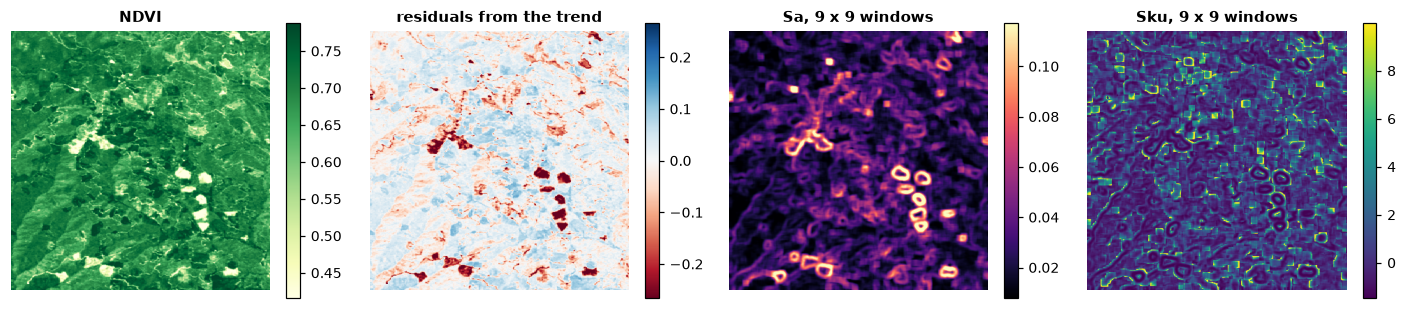
NDVI, its residuals, and Sa and Sku in 9 x 9 windows

Sa is highest where the window straddles the edge of a clearing (the rings around the dark patches of the residuals) and low inside even stands; Sku is highest where a few cells stand out from an even background, just outside those edges and in scattered gaps. Windows run in parallel; extremes and peak counts take shortcuts, the other metrics are computed on each window as on a raster.

Spatial structure¶

The autocorrelation function (aacf) and the Fourier spectrum of a surface describe its spatial structure:

print(ls.surface.scl(z).round(1))        # fastest and slowest decay to 0.2 and 1/e (m)
print(ls.surface.stxr(z).round(3))       # texture aspect ratio: 0 oriented, 1 isotropic
print(ls.surface.std(z).round(3))        # texture direction (degrees) and its index
print(ls.surface.srw(z).round(1))        # dominant radial wavelength, index, half-power wavelength
print(round(ls.surface.sfd(z), 4))       # fractal dimension

[ 247.8  164.8 6873.  6873. ]
[0.036 0.024]
[90.     0.197]
[4.0970e+02 6.0000e-01 1.6387e+03]
2.0001

Distances are in map units, metres on longitude/latitude rasters like this one. The correlation lengths say how far one must move for the surface to be unrelated to itself; their ratio, whether the texture is stretched in one direction.

Terrain indices¶

A DEM is a surface too, with indices of its own:

dem = ls.load_raster(ls.surface.example_data("orelevation"))
slope = ls.surface.terrain(dem, "slope")               # degrees, Horn's method
aspect = ls.surface.terrain(dem, "aspect")
tpi = ls.surface.tpi(dem, 15)                          # elevation minus the 15 x 15 mean
tri = ls.surface.tri(dem)                              # terrain ruggedness
vrm = ls.surface.vrm(dem, 5)                           # vector ruggedness
hli = ls.surface.hli(aspect, slope, scaled=True)       # heat load (latitude from the raster)
curv = ls.surface.curvature(dem, "profile")
for name, v in [("slope", slope), ("tpi", tpi), ("tri", tri), ("vrm", vrm), ("hli", hli)]:
    print(name, round(float(v.mean()), 3), round(float(v.max()), 3))
ls.plot([dem, slope, tpi])     # one map, a layer each
ls.write_raster(slope, "slope.tif")

slope 18.454 62.107
tpi 0.178 60.898
tri 23.148 141.534
vrm 0.012 0.165
hli 0.771 1.072

Elevation, slope, topographic position and heat load

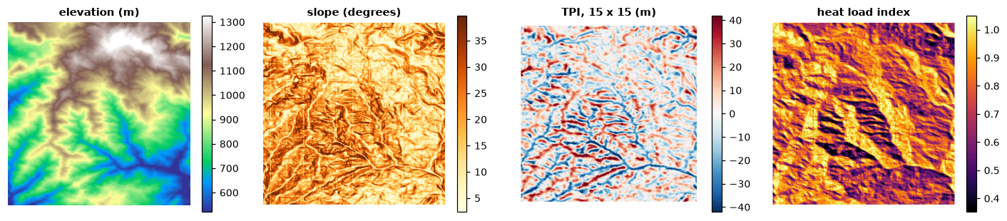
TPI is positive on ridges and hilltops, negative in valleys; its multi-scale sum hsp gives a hierarchical slope position.
TRI and VRM measure ruggedness: TRI from elevation differences, VRM from the dispersion of the surface's normal vectors, so a steep but even slope is not rugged.
Heat load (McCune & Keon 2002) combines slope, aspect folded about the warmest direction (south-west in the northern hemisphere) and latitude.
curvature, srr, dissection, spherical_sd and trasp complete the set.

Landforms¶

Geomorphons (Jasiewicz & Stepinski 2013) classify each cell into one of ten landforms by looking along eight lines of sight up to a search distance: whether the terrain rises, falls or stays level in each direction. Unlike slope or curvature from a 3 x 3 window, they capture the form of the site at the scale of the search, and make expressive covariates for species distribution and land change models. They need a projected DEM:

utm = ls.reproject(ls.load_raster(ls.surface.example_data("orelevation")), "EPSG:32610", res=30)
forms = ls.surface.geomorphons(utm, search=20)
print(forms.share()[["name", "share"]].round(3).to_string())

           name  share
form                  
1          flat  0.000
2          peak  0.014
3         ridge  0.110
4      shoulder  0.003
5          spur  0.215
6         slope  0.363
7        hollow  0.182
8     footslope  0.004
9        valley  0.098
10          pit  0.011

Slopes, spurs and hollows dominate these mountains. forms.ternary keeps the pattern of each cell (one of 498), and measures=True adds intensity, exposition, range and the shape of each geomorphon. The forms are GRASS GIS's r.geomorphon bit for bit, with its errors corrected.

Hilltop protection areas¶

Brazil's Forest Code (Lei 12.651/2012) protects the tops of hills at least 100 m high with a mean slope above 25°: the area above two thirds of their height, measured from the base (the plain or water around them, or the saddle where they meet higher ground). hilltop finds every summit with its base and marks the protected area of those that qualify:

h = ls.surface.hilltop(dem)
hills = h.hills[h.hills.qualifies]
print(hills[["top", "base", "base_kind", "height", "mean_slope", "threshold", "app_cells"]].round(1))
print(len(h.hills), "summits")
conama = ls.surface.hilltop(dem, min_height=50, min_slope=16.7, slope="line")   # CONAMA 303/2002
print(int(conama.hills["qualifies"].sum()), "hills,", int(conama.app.sum()), "cells with the older rule")
ls.plot([dem, h.app])

         top   base base_kind  height  mean_slope  threshold  app_cells
hill
208   1068.0  909.0    saddle   159.0        25.6     1015.0        115
625 summits
12 hills, 1400 cells with the older rule

Of 625 summits, one is a hill for the law: 159 m above the saddle that joins it to higher ground, with a mean slope of 25.6°. The rest are bumps on larger landforms or too gentle; the highest summit of the map stands 957 m above the lowest point but its slopes average 18°. Give the plains and water bodies around the hills as plain= (a mask) so that their bases are taken from them. The older rule of CONAMA 303/2002 (50 m, a slope of 30 % along the line from the summit to its foot) finds twelve hills here. Bases, heights and slopes depend on the DEM's resolution and accuracy: the result is a starting point for field and legal work.

Validation¶

Every metric is checked in the test suite against R: against geodiv and spatialEco (with terra) themselves where they are right, and where they err against their code with the error corrected. The corrections cover the root mean square height and the moments built on it, the seven-point slopes, the valley search, the summit curvature, the bearing area curve's areas, the centre of the Fourier images, the fractal dimension's prisms, the choice of trend surface, curvature's second derivatives, hsp's z-scores and the heat load's southern hemisphere; see the benchmarks and each function's notes. Typical gains in speed are tens to thousands of times over the R packages. hilltop follows the law rather than a program (Dinamica EGO's CalcHilltop applies the older CONAMA rule with other definitions); it is checked against an independent computation of the landforms on random DEMs and on cones and ranges of known geometry.