Chapter 8

Circuit theory

What does an electrical circuit have to do with a deer crossing a valley? More than it seems. In 2006, the geneticist Brad McRae showed that genetic differentiation between populations is predicted by the effective resistance of the landscape between them, computed exactly as an engineer computes the resistance of a network of resistors (McRae, 2006). The reason is a deep mathematical link between electric current and random walks. Since then, circuit theory has become one of the main tools of connectivity science (McRae et al., 2008; Dickson et al., 2019).

In this chapter

• the correspondence between random walkers and electric circuits;
• Ohm's law, resistors in series and in parallel, effective resistance;
• why redundant routes matter, and what least-cost paths miss;
• current density, pinch points and barriers;
• pairwise, advanced, one-to-all and omnidirectional analyses, and how to read them.

From random walkers to circuits

Imagine an animal that does not know the landscape. At every step it moves to a neighbouring cell, choosing more often the cells that are easier to cross. This is a random walk on the landscape, weighted by the conductance of each cell (the inverse of its resistance). Doyle and Snell (1984) showed that such random walks and electric circuits obey the same equations:

Random walk	Electric circuit
ease of moving between two cells	conductance (1 / resistance)
probability that a walker starting at a cell reaches A before B	voltage at the cell, with A at 1 V and B grounded
net number of times walkers pass through a cell going from A to B	current through the cell
expected time to go from A to B and back (commute time)	proportional to the effective resistance between A and B

Every result about current therefore has a meaning in terms of movement. The current through a cell is the expected net number of passages of a walker moving from the source to the ground: where current is high, movement is funnelled.

Ohm's law and effective resistance

A resistor of resistance R carrying a current I has a voltage V = R I across it (Ohm's law). Resistors combine in two ways:

series: R = R₁ + R₂        parallel: 1/R = 1/R₁ + 1/R₂ In series, resistances add: a longer route is harder. In parallel, conductances add: a second route makes the connection easier.

The effective resistance between two nodes of a network is the single resistance that would carry the same current for the same voltage. It combines the length of the routes (series) and their number and width (parallel). Here is a chain of two links of resistance 1, then the same chain with a second, parallel route:

import numpy as np
import landschaft as ls
from landschaft import circuit

one_route = [[1, 2, 1.0], [2, 3, 1.0]]                       # 1 - 2 - 3
two_routes = one_route + [[1, 4, 1.0], [4, 3, 1.0]]          # and 1 - 4 - 3

r1 = circuit.circuitscape_network_pairwise(one_route, [1, 3]).resistances[1, 2]
r2 = circuit.circuitscape_network_pairwise(two_routes, [1, 3]).resistances[1, 2]
{"one route": r1, "two routes": r2}

The second route halves the effective resistance, while the least-cost distance (the cheapest single route, 2 in both cases) does not change. This is the key difference between the two approaches: circuit theory rewards redundancy. Wide corridors and multiple routes are better connected than a single thin corridor of the same length, which matches our intuition about how populations exchange individuals and genes (McRae & Beier, 2007).

Commute time

The correspondence can be checked directly. For a network with m links of unit resistance, the expected commute time between two nodes (the number of steps a random walker needs to go from one to the other and back) is 2 m times their effective resistance (Chandra et al., 1996). In the square network above, m = 4 and the effective resistance is 1, so the commute time should be 8 steps. A simulation:

rng = np.random.default_rng(0)
neighbours = {1: [2, 4], 2: [1, 3], 3: [2, 4], 4: [1, 3]}


def commute_time(start, target):
    node, steps, reached = start, 0, False
    while True:
        node = neighbours[node][rng.integers(2)]
        steps += 1
        if node == target:
            reached = True
        elif reached and node == start:
            return steps


round(float(np.mean([commute_time(1, 3) for _ in range(20_000)])), 2)

The walkers need 8 steps on average, as the circuit predicts. In Landschaft, HabitatGraph.from_raster(..., distance="commute-time") uses this quantity as the distance between habitat patches (chapter 7).

Current on a landscape: pinch points

On a raster, every cell is a node connected to its neighbours by resistors of the cells' resistances. Consider a simple landscape: open land of uniform resistance crossed by an impassable wall with two gaps, a narrow one (3 cells) and a wide one (18 cells). Current flows from a line of cells on the left to a line on the right:

resistance = np.ones((60, 100))
resistance[:, 48:52] = np.nan          # NaN: impassable wall
resistance[8:11, 48:52] = 1.0          # narrow gap, 3 cells
resistance[34:52, 48:52] = 1.0         # wide gap, 18 cells

points = np.zeros(resistance.shape)
points[25:35, 5] = 1                   # focal region 1, on the left
points[25:35, 94] = 2                  # focal region 2, on the right

flow = circuit.circuitscape_pairwise(resistance, points, cum_map=True)
current = np.asarray(flow.cum_current)

narrow = np.nansum(current[8:11, 50])
wide = np.nansum(current[34:52, 50])
{"share through narrow gap": narrow / (narrow + wide),
 "current per cell, narrow": current[8:11, 50].mean(),
 "current per cell, wide": current[34:52, 50].mean()}

Now the single best route:

open_land = np.where(np.isnan(resistance), 0, resistance)      # 0: impassable here
path = ls.least_cost_path(open_land, points == 1, points == 2)
rows_crossed = np.flatnonzero(np.asarray(path.lcp_mask)[:, 50])
rows_crossed

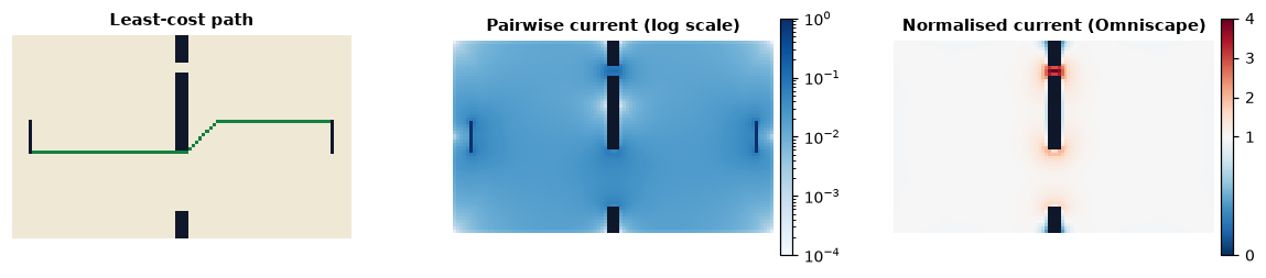
The least-cost path goes through the wide gap and ignores the narrow one entirely. Circuit theory sends about a quarter of the flow through the narrow gap, which holds only a seventh of the gap width, so the current per cell there is about twice as high: a pinch point. If the narrow gap were closed, a quarter of the movement would have to find another way. Pinch points are where corridors are most vulnerable and where protection or restoration is most efficient (McRae et al., 2008).

The modes of a circuit analysis

Mode	Current flows	Answers	Tool
pairwise	between every pair of focal points or regions, one pair at a time	effective resistance between all pairs (an isolation matrix), cumulative current	circuit.circuitscape_pairwise
advanced	from sources you place to grounds you place	flow between specific areas, e.g. from a population to all suitable habitat	circuit.circuitscape_advanced
one-to-all / all-to-one	from each point to all others (or the reverse)	how connected each point is to the rest	circuit.circuitscape_one_to_all
omnidirectional	between all cells within a moving window	connectivity everywhere, without choosing points	ls.omniscape

These are the modes of the Circuitscape software (Shah & McRae, 2008; Anantharaman et al., 2020), whose results Landschaft reproduces. The pairwise resistance matrix can be compared with genetic distances between populations (isolation by resistance; McRae, 2006; McRae & Beier, 2007). The cumulative current map highlights corridors and pinch points between the chosen points. Networks given as lists of links, rather than rasters, are analysed with circuitscape_network_pairwise and circuitscape_network_advanced.

Omnidirectional connectivity

Choosing focal points biases the result towards them: corridors appear between the chosen reserves and nowhere else. Omniscape avoids the choice (McRae et al., 2016; Landau et al., 2021). A circular window of a given radius moves over the landscape; in each window, current flows from every source cell towards the centre, and the currents of all windows are summed. Sources are usually the cells of good habitat, with strength proportional to their quality. The result, the cumulative current, maps how much movement every cell carries between all places within the radius.

Cumulative current is high where movement concentrates, but also simply where there are many sources. The flow potential, the current the same sources would produce in a landscape of uniform resistance, is the baseline; their ratio, the normalised current, reads:

Normalised current	Reading
well above 1	movement is channelised: more flow than expected, corridors and pinch points
about 1	diffuse flow, as in an unobstructed landscape
well below 1	movement is impeded: barriers, or areas avoided

omni = ls.omniscape(resistance, radius=15, block_size=1,
                    flow_potential=True, normalized_current=True)
normalised = np.asarray(omni["normalized_cum_currmap"])
{"narrow gap": np.nanmean(normalised[8:11, 48:52]),
 "wide gap": np.nanmean(normalised[34:52, 48:52]),
 "open land": np.nanmean(normalised[:, 20])}

With no focal points at all, the omnidirectional analysis finds the same pinch point: in the narrow gap the flow is more than three times what an unobstructed landscape would carry, in the wide gap somewhat more, and in the open land about as expected.

The radius plays the role of the dispersal distance (chapter 2): choose it from the species' movement ability. The block_size option solves one window per block of cells, which speeds up large analyses considerably with little effect on the result.

When to use circuit theory

Use it when:

• the movement of interest is exploratory (dispersal of juveniles, gene flow over generations) rather than directed by knowledge of the landscape;
• redundancy matters: wide corridors and multiple routes should count more than a single thin path;
• you need to find pinch points and barriers, or to map connectivity everywhere (omnidirectional).

Prefer least-cost analysis (chapter 9) when you need a single corridor to delineate or restore, or when animals move with knowledge of the landscape (seasonal migration). Prefer graph indices (chapter 7) to rank patches by their contribution to reachable habitat. As in every resistance-based model, the result is only as good as the resistance surface (chapter 6).

Key points

• Random walks on a landscape and electric current obey the same equations; current measures the net passage of random walkers.
• Effective resistance combines the length and the number of routes; parallel routes lower it, unlike least-cost distance.
• High current density marks pinch points, where movement is funnelled and most vulnerable.
• Pairwise and advanced modes connect chosen places; omnidirectional analysis maps connectivity everywhere; normalised current separates channelised from diffuse and impeded flow.

Check your understanding

1. Two reserves are joined by one corridor. A second, identical corridor is restored in parallel. What happens to their effective resistance and to their least-cost distance?
2. A cell has a very high cumulative current in an omnidirectional map, but a normalised current of 1. How do you interpret it?
3. Why is current density higher in a narrow gap than in a wide one?

Answers

1. The effective resistance halves (two equal resistances in parallel); the least-cost distance does not change, since the best single route is the same.
2. Much movement passes through it, but no more than the same sources would produce in an unobstructed landscape: it is a busy area because of its many sources, not a bottleneck.
3. The same flow must cross fewer cells, so each cell carries more of it, as water speeds up in a narrow section of a river.

References

• Anantharaman, R., Hall, K., Shah, V. B., & Edelman, A. (2020). Circuitscape in Julia: high performance connectivity modelling to support conservation decisions. Proceedings of the JuliaCon Conferences, 1(1), 58.
• Chandra, A. K., Raghavan, P., Ruzzo, W. L., Smolensky, R., & Tiwari, P. (1996). The electrical resistance of a graph captures its commute and cover times. Computational Complexity, 6, 312–340.
• Dickson, B. G., Albano, C. M., Anantharaman, R., et al. (2019). Circuit-theory applications to connectivity science and conservation. Conservation Biology, 33(2), 239–249.
• Doyle, P. G., & Snell, J. L. (1984). Random Walks and Electric Networks. Mathematical Association of America.
• Landau, V. A., Shah, V. B., Anantharaman, R., & Hall, K. R. (2021). Omniscape.jl: software to compute omnidirectional landscape connectivity. Journal of Open Source Software, 6(57), 2829.
• McRae, B. H. (2006). Isolation by resistance. Evolution, 60(8), 1551–1561.
• McRae, B. H., & Beier, P. (2007). Circuit theory predicts gene flow in plant and animal populations. Proceedings of the National Academy of Sciences, 104(50), 19885–19890.
• McRae, B. H., Dickson, B. G., Keitt, T. H., & Shah, V. B. (2008). Using circuit theory to model connectivity in ecology, evolution, and conservation. Ecology, 89(10), 2712–2724.
• McRae, B. H., Popper, K., Jones, A., et al. (2016). Conserving Nature's Stage: Mapping Omnidirectional Connectivity for Resilient Terrestrial Landscapes in the Pacific Northwest. The Nature Conservancy, Portland, Oregon.
• Shah, V. B., & McRae, B. H. (2008). Circuitscape: a tool for landscape ecology. In Proceedings of the 7th Python in Science Conference (pp. 62–65).