

Animal movement, part 2 of 5
Clean tracks and measure them
Remove the records Movebank hides and the duplicated times, measure every step's distance, time lag, speed, direction and turn, find the errors the measures reveal, and see how the sampling interval changes them.
- Level
- Beginner
- Time
- 45 min
Raw tracks contain records that should not be analysed: locations flagged as outliers, the same time recorded twice, fixes whose error is larger than the step they belong to. In this part you will clean the fishers' tracks from part 1 with Movebank's own flags and with move2's filters, then measure each step: its length, its duration, its speed, its direction and the turn the animal made. The measures are the first summary of how an animal moves, and also the best test of the data: an impossible speed is usually an error. At the end you will have every location of the fishers with its five measures, the steps as lines, and a clear sense of how much the sampling interval changes what you measure.
The idea#
Errors in tracking data#
A GPS location is an estimate. In the open, a modern receiver places itself within a few metres; under a dense canopy, near cliffs or with few satellites in view, the error grows to tens of metres, and now and then a fix is hundreds of metres or kilometres off (Frair et al., 2010). Three kinds of problem are common:
- Outliers: a location far from those before and after it, reached at an impossible speed and left at once. The track shows a spike: out and straight back.
- Duplicates: two records with the same time, from a device that sent a record twice, from two files appended, or from a sensor that logs the time with too coarse a resolution.
- Imprecise locations: no single location is wrong by much, but when the animal rests, its locations scatter around the spot where it lies, and the track zig-zags without the animal moving.
Bjørneraas et al. (2010) screened GPS data by the movement they imply: a location is suspect when the speeds
to and from it are both high and the turn at it is close to 180°. Movebank lets researchers flag such records
(by hand, or with its filters) and hides them from the default view: the column visible says which are shown.
The measures of a step#
Key idea: measuring a step on the Earth
Movebank's locations are in longitude and latitude, angles on the Earth, not distances. A degree of longitude near Albany (42.8° N) is 82 km, but 111 km at the equator; Terraflux measures on the Earth itself instead of on a flat map:
-
Distance (
move.distance): the great-circle distance between two locations on a sphere of radius \( R = 6\,371\,010 \) m, as move2 computes it (with the s2 geometry library),\[ d = 2R \arcsin \sqrt{\sin^2\frac{\varphi_2 - \varphi_1}{2} + \cos\varphi_1 \cos\varphi_2 \sin^2\frac{\lambda_2 - \lambda_1}{2}} \]where \( \varphi \) is the latitude and \( \lambda \) the longitude, in radians.
-
Time lag (
move.time_lags): the time to the next location, exact to the nanosecond. - Speed (
move.speed): distance over time lag, the average speed along the straight line between the two locations. - Azimuth (
move.azimuth): the direction of the step, clockwise from north (0° north, 90° east, ±180° south), the geodesic azimuth on the WGS 84 ellipsoid (Karney, 2013). - Turn angle (
move.turn_angle): the azimuth of the step leaving a location minus that of the step arriving, between -180° and 180°; positive is a turn to the right.
In a projected coordinate system (metres on a flat map), the same nodes measure straight lines and angles on the grid instead.
Each measure belongs to a location and describes the step that leaves it: the distance from this location to the next, the time until the next. The last location of each track has no next one, so its measures are missing (NaN); the turn angle is missing at the first location too, which has no step arriving.
The interval shapes the measures#
A track samples a continuous path. Between two fixes the animal followed some winding route, and the straight line between the fixes is shorter. The longer the interval, the more of the path is cut: distances and speeds shrink as the interval grows, and turns look more random, because over a long interval the animal may have turned several times. Rowcliffe et al. (2012) showed with camera-trap and GPS data that a daily distance estimated from hourly fixes can be half the true one. The opposite error appears at very short intervals: the location error becomes comparable to the step itself, and the measured distance adds the error's zig-zag to the real movement.
Measures are therefore never a property of the animal alone, but of the animal at a sampling interval. Report the
interval with them, and compare animals only at a common interval: move.filter_per_interval (below) and
move.resample (part 4) make one.
When to use it#
- Always, before any analysis: the filters remove what should not be analysed, and the measures reveal what the filters missed (impossible speeds, spikes).
- To describe movement: how far an animal travels in a day, how fast, how straight.
- To compare individuals, seasons or sexes, at a common sampling interval.
- To prepare variables for other analyses: speeds and turn angles are the inputs of behavioural segmentation (resting, foraging, travelling) and of step selection functions (part 5).
The measures are descriptive. For the distribution of step lengths and turn angles, fitted as parametric distributions, see part 5; for the area an animal uses, see part 4's summaries.
What you need#
The tracks read in part 1, with the records without a location removed. The measures need the records of each animal ordered by time and without repeated times (a speed over a time lag of zero is infinite), which the filters below make sure of.
Build the model#
Clean#
Model file (TOML)
format = "terraflux/1"

[[nodes]]
id = "read"
op = "move.read_tracks"
params = { path = "fishers.csv.gz" }

[[nodes]]
id = "located"
op = "vector.filter"
inputs = { vector = "read.tracks" }
params = { expression = "not isnull(geometry.x)" }

[[nodes]]
id = "visible"
op = "move.filter_movebank_visible"
inputs = { tracks = "located.vector" }
note = "Movebank's outliers out"

[[nodes]]
id = "unique"
op = "move.filter_unique"
inputs = { tracks = "visible.tracks" }
note = "One record per time and animal"
-
Read and keep the located records as in part 1 (nodes 1 and 2).
-
Keep the records Movebank shows with
move.filter_movebank_visible(library subject Animal movement), connected tolocated.vector. When the file has the columnvisible, the node keeps the records where it is true. A file without it (an older export, a table of your own) is filtered by the outlier columns instead: the records marked as outliers by hand, by an algorithm or on import are dropped, unless a person marked them valid. This is move2'smt_filter_movebank_visible. -
Remove the duplicated times with
move.filter_unique, connected tovisible.tracks. Of the records of one animal that share a time, the node keeps the one that holds the most: with the defaultcriterion = "subsets", a record is dropped when each of its values equals the other's or is missing (it repeats it, or holds less). When two records at the same time disagree (two different locations), neither is a subset of the other, and the node keeps both and warns: decide which one to keep by another rule, withcriterionfirst,lastorsample(one at random, as R'ssample.intafterset.seed(seed), the same record move2 keeps).columns_alsonames more columns that must match for two records to be duplicates, such as a sensor type when a file mixes sensors.
On the fishers, neither filter removes anything: all 32,904 located records are visible, and no animal has two records at the same time. This is the case with most published data, which the authors have cleaned; with data straight from a collar it is not. The nodes cost nothing, and a model that keeps them works on the next data set too.
Measure#
Model file (TOML)
format = "terraflux/1"

[[nodes]]
id = "read"
op = "move.read_tracks"
params = { path = "fishers.csv.gz" }

[[nodes]]
id = "located"
op = "vector.filter"
inputs = { vector = "read.tracks" }
params = { expression = "not isnull(geometry.x)" }

[[nodes]]
id = "visible"
op = "move.filter_movebank_visible"
inputs = { tracks = "located.vector" }

[[nodes]]
id = "unique"
op = "move.filter_unique"
inputs = { tracks = "visible.tracks" }

[[nodes]]
id = "lags"
op = "move.time_lags"
inputs = { tracks = "unique.tracks" }
params = { units = "min" }

[[nodes]]
id = "dist"
op = "move.distance"
inputs = { tracks = "lags.tracks" }

[[nodes]]
id = "speed"
op = "move.speed"
inputs = { tracks = "dist.tracks" }
params = { units = "km/h" }

[[nodes]]
id = "heading"
op = "move.azimuth"
inputs = { tracks = "speed.tracks" }
params = { units = "deg" }

[[nodes]]
id = "turn"
op = "move.turn_angle"
inputs = { tracks = "heading.tracks" }
params = { units = "deg" }
The five measures are chained: each node takes the tracks, adds one column and gives them on, so the last node's
tracks hold all five. The order does not matter. Each has a units setting and a column setting (the name of
the column it adds; by default time_lag, distance, speed, azimuth, turn_angle):
move.time_lags:unitss (the default), min, h or d.move.distance: m (the default in longitude and latitude) or km. In a projected system the distance is in the system's units.move.speed: m/s, km/h, m/h or km/d; by default metres per second.move.azimuthandmove.turn_angle: rad (the default, as in move2) or deg.
Every node also gives a table of the attributes that are numbers, for table.write or a chart.
Steps as lines#
Model file (TOML)
[[nodes]]
id = "turn"
op = "move.turn_angle"
inputs = { tracks = "heading.tracks" }
params = { units = "deg" }

[[nodes]]
id = "segments"
op = "move.segments"
inputs = { tracks = "turn.tracks" }
move.segments turns each location into a two-point line, from it to the next location of the same animal,
with all the location's attributes. Coloured by speed, the lines show where an animal ran and where it lingered;
selected by a polygon (with vector.spatial_join or vector.clip), they show where it crossed a road or a
river. The last location of each track has no step and stays a point.
One location per interval#
Model file (TOML)
[[nodes]]
id = "unique"
op = "move.filter_unique"
inputs = { tracks = "visible.tracks" }

[[nodes]]
id = "thin"
op = "move.filter_per_interval"
inputs = { tracks = "unique.tracks" }
params = { unit = "30 mins", criterion = "first" }
move.filter_per_interval keeps one location per interval of time: unit is the interval (15 mins,
hour, 2 hours, day, week, month...), and criterion which location of each interval to keep:
first (the default), last or random. The intervals are those of the calendar, as R's lubridate cuts them:
30 mins means from :00 to :29 and from :30 to :59 of every hour, day from midnight to midnight (UTC), week
from Sunday. The result is a track with at most one location per interval, but not a regular one: an interval
without a fix gives none. For steps of a regular interval, see move.resample in part 4.
Read the results#
The sampling schedules#

The histogram of the time lags is the best summary of a data set's sampling. Here there are three schedules: five animals at 2 minutes (F2, F3, M3, M4, M5), two at 10 (F1, M2) and one at 15 (M1). The smaller peaks are the schedule's multiples, where one or more fixes in a row failed, and the long tail (up to two days for M3) are the gaps when the collar found no satellites for hours. At the other end, 933 steps are shorter than a minute: fixes taken in quick succession.
Impossible speeds#
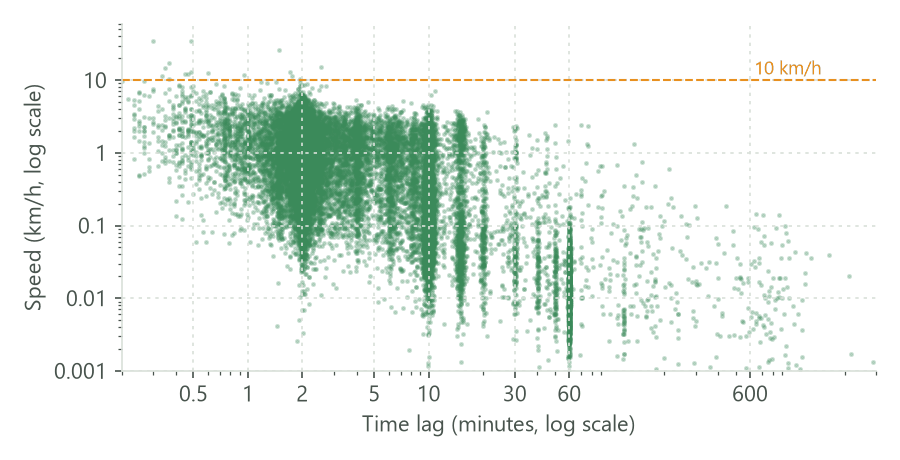
Fishers can run, but not for long: a speed above 10 km/h sustained for minutes is unlikely. Only 19 steps are faster than that, and 14 of them last less than a minute. These are not sprints: two fixes a few seconds apart differ by their errors, a few tens of metres, and divided by a few seconds that becomes a high speed. The figure shows the general pattern: the shorter the time lag, the wider the spread of the speeds, because the error weighs more. At lags of an hour and more, the speeds are low, both because the fisher rested and because the straight line cuts its route.
The usual remedy follows from the figure: do not compute speeds over very short lags. Thin the tracks to one location per interval (below) or resample them (part 4) before measuring speeds, and screen the steps above a plausible speed by eye, on the map, before removing them.
Each animal#
| animal | median lag (min) | median speed (km/h) | 99th percentile (km/h) | km per day | km per day at 10 min |
|---|---|---|---|---|---|
| F1 | 10 | 0.14 | 2.9 | 5.98 | 5.98 |
| F2 | 2 | 0.99 | 4.7 | 9.84 | 7.45 |
| F3 | 2.1 | 0.82 | 4.6 | 4.8 | 3.4 |
| M1 | 15 | 0.1 | 3.1 | 8.22 | 8.22 |
| M2 | 10 | 0.17 | 3.7 | 7.49 | 7.49 |
| M3 | 2.2 | 0.99 | 4.9 | 7.51 | 6.11 |
| M4 | 2 | 0.69 | 4.8 | 7.51 | 5.26 |
| M5 | 2 | 0.88 | 4.6 | 9.03 | 6.27 |
The table shows the trap of comparing measures across schedules. The median speed of the animals fixed every 2 minutes is four to ten times that of the animals fixed every 10 or 15. Part of this is the interval, and part is when the fixes were taken: the 2-minute collars obtained many more fixes while the animals moved than while they rested (the night of M4 in part 1), so their median step is a moving step, while the slower schedules sampled resting and moving more evenly. The distance per day depends on the interval too: at their own rate, the 2-minute animals travelled 4.8 to 9.8 km a day; with one location per 10 minutes, 3.4 to 7.5 km. Only the last column compares the eight animals on the same footing, and even it pools winter and spring of different years.
A night of steps#

The segments of M4's night (the same day as in part 1) show travel at 2 to 5 km/h along fairly straight lines, and slow, tangled steps where it lingered. A long straight step with a low speed is a warning sign of a gap: the fisher did not walk that line slowly, the collar simply missed it.
Turns#

The rose diagrams show the share of turn angles in each 15° class. With one location every 2 minutes, two peaks stand out: near 0°, where the fisher kept going straight, and near 180°, where the track went back on itself. Most reversals are the zig-zag of the location error while the animal rested. At 30 minutes, the forward peak fades; at 2 hours the turns are almost uniform, apart from the reversals of an animal that went somewhere and came back. The persistence of a movement, its tendency to keep its direction, is a property of a time scale: fishers move persistently over minutes, not over hours.
Settings that change the answer#
The interval of move.filter_per_interval changes everything measured after it. Here is M4's night of part
1 with one location per interval, from 2 minutes to 2 hours:


From 2 minutes to 2 hours, the distance travelled that night falls from 12.7 to 4.5 km. Neither is the true distance: the 2-minute track adds the error's zig-zag, the 2-hour track cuts every loop. A distance per day is meaningful only with its interval, and the comparison of distances only at a common one.
The other settings change little but the presentation: units of each measure, and criterion of the filters
(for move.filter_per_interval, last or random instead of first move each location within its
interval; random with a different seed gives a different track).
Common pitfalls#
- Measuring before cleaning. A duplicated time gives a time lag of zero and an infinite speed:
move.speedstops with an error and namesmove.filter_unique. Records without a location stop every measure; drop them first. - Radians by default.
move.azimuthandmove.turn_anglegive radians, as move2 does; setunits = "deg"for degrees. - Directions differ between packages. Azimuths here are clockwise from north (move2's convention). amt's steps (part 4) give directions anticlockwise from east, as mathematics does. Do not mix the two.
- The measure belongs to the step leaving the location. When you join measures to the habitat, the location's habitat is where the step started. Part 5 extracts the habitat at the end of each step instead.
- Speeds over short lags. Most extreme speeds in GPS data are errors over steps of seconds. Look at speed against time lag before deciding on a threshold.
- Comparing across schedules. Distances, speeds and turns of animals fixed at different intervals are not comparable; thin or resample them to a common one first.
Going further#
- Projections, interpolation and simulated tracks: measure in metres on a local projection, fill gaps, and compare with tracks of random motion.
- Regular steps and track summaries:
move.resamplefor steps of a regular interval, and summaries of each track. - The operators' reference:
move.filter_movebank_visible,move.filter_unique,move.filter_per_interval,move.time_lags,move.distance,move.speed,move.azimuth,move.turn_angle,move.segments.
References#
- Bjørneraas, K., Van Moorter, B., Rolandsen, C. M., & Herfindal, I. (2010). Screening Global Positioning System location data for errors using animal movement characteristics. Journal of Wildlife Management, 74(6), 1361-1366. https://doi.org/10.2193/2009-405
- Frair, J. L., Fieberg, J., Hebblewhite, M., Cagnacci, F., DeCesare, N. J., & Pedrotti, L. (2010). Resolving issues of imprecise and habitat-biased locations in ecological analyses using GPS telemetry data. Philosophical Transactions of the Royal Society B, 365(1550), 2187-2200. https://doi.org/10.1098/rstb.2010.0084
- Karney, C. F. F. (2013). Algorithms for geodesics. Journal of Geodesy, 87(1), 43-55. https://doi.org/10.1007/s00190-012-0578-z
- Kranstauber, B., Safi, K., & Scharf, A. K. (2024). move2: R package for processing movement data. Methods in Ecology and Evolution, 15(9), 1561-1567. https://doi.org/10.1111/2041-210X.14383
- Rowcliffe, J. M., Carbone, C., Kays, R., Kranstauber, B., & Jansen, P. A. (2012). Bias in estimating animal travel distance: the effect of sampling frequency. Methods in Ecology and Evolution, 3(4), 653-662. https://doi.org/10.1111/j.2041-210X.2012.00197.x