IIC, PC and the equivalent connected area

In part 1 the forests around Hannover became a graph, and we counted its links and components. Counts say little about what matters to a species: how much habitat it can actually reach. In this part you compute the indices that answer that question, the integral index of connectivity (IIC) and the probability of connectivity (PC), first on a toy landscape of four patches that you can check by hand, then on the 154 forest patches at thirteen dispersal distances. You will turn them into the number most studies report, the equivalent connected area (ECA) in hectares, and split it into the habitat a species finds inside patches, through direct moves, and through stepping stones. At the end you will have a curve of connectivity against dispersal distance for the landscape, and you will know how to read and report it.

The idea#

Connectivity as reachable habitat#

By the early 2000s dozens of connectivity indices had been proposed, and many behaved strangely: some could rise when a patch was destroyed, others ignored the size of the patches, or only counted links. Pascual-Hortal and Saura (2006) listed the properties a good index should have, the most important being that losing habitat must never increase connectivity, and found that most of the existing indices failed some of them. They proposed the integral index of connectivity, and a year later Saura and Pascual-Hortal (2007) its probabilistic version, the probability of connectivity. Both rest on one idea: habitat availability. A landscape is well connected for a species if the habitat it can reach, from wherever it is, is large; a patch counts both for the habitat it holds and for the habitat it gives access to.

Key idea: the probability of connectivity

For \(n\) patches with areas \(a_i\) in a study area of area \(A_L\),

\[ \mathrm{PC} = \frac{\sum_{i=1}^{n}\sum_{j=1}^{n} a_i\, a_j\, p^*_{ij}}{A_L^2} \]

\(p_{ij}\) is the probability of moving directly from \(i\) to \(j\), from the dispersal kernel (part 1): \(p_{ij} = p^{\,d_{ij}/d}\), with \(p\) the probability at the distance \(d\).
\(p^*_{ij}\) is the probability of the best path from \(i\) to \(j\): the largest product of the \(p\) of its steps, which may go through other patches. For \(i = j\), \(p^*_{ii} = 1\).
PC is the probability that two points dropped at random in the study area both fall in habitat and are connected. It is 0 without habitat and 1 when the whole area is one patch.

The integral index of connectivity is the same with links instead of probabilities: \(\mathrm{IIC} = \sum_i \sum_j a_i a_j / (1 + nl_{ij}) / A_L^2\), where \(nl_{ij}\) is the number of links on the shortest path between \(i\) and \(j\) (and \(1/(1+nl_{ij}) = 0\) when no path joins them). It is the choice for a threshold distance, PC for a kernel.

The equivalent connected area#

PC and IIC are small numbers that depend on the size of the study area: doubling the area of farmland around the same forest divides PC by four. Saura et al. (2011) proposed to report instead the square root of the numerator, the equivalent connected area (ECA, called EC(PC) and EC(IIC) by Conefor and Terraflux):

\[ \mathrm{ECA} = \sqrt{\textstyle\sum_i \sum_j a_i\, a_j\, p^*_{ij}} \]

ECA is an area, in the units of the patches' areas: the size of a single patch that would offer the same amount of reachable habitat as the whole network. It has two easy bounds:

if nothing is connected (\(p^*_{ij} = 0\) between patches), ECA is \(\sqrt{\sum_i a_i^2}\), dominated by the largest patch;
if everything is perfectly connected (\(p^*_{ij} = 1\)), ECA is the total habitat area \(\sum_i a_i\).

So ECA divided by the habitat area says how much of the habitat is "functionally one": a useful number to compare dates (connectivity lost faster or slower than habitat) and regions.

Three ways to reach habitat#

The numerator of PC adds terms of three kinds, and Saura and Rubio (2010) proposed to report their shares as fractions:

intra (\(i = j\)): the habitat inside each patch, \(a_i^2\). A species that never leaves its patch still has this.
direct (\(i \ne j\), the best path is the direct move): habitat reached by crossing one gap.
step (\(i \ne j\), the best path goes through other patches): habitat reached only thanks to stepping stones in between.

A landscape whose connectivity is mostly intra depends on its large patches; one with a large step fraction depends on small patches that relay movement, and is fragile if they are lost.

A toy landscape by hand#

Four patches of 100, 50, 20 and 80 ha in a landscape of 10,000 ha, with the gaps between them, for a species half of whose dispersers cross 1 km (\(p = 0.5\) at \(d = 1000\) m):

Four patches and the probability of moving directly between each pair — The toy landscape. Each line is labelled with the gap and the direct probability p = 0.5^(gap / 1 km); thicker lines are likelier moves. From patch 1 to patch 3, going through patch 2 (0.57 × 0.66 = 0.38) beats the direct move (0.35): patch 2 is a stepping stone.

Without any movement, ECA would be \(\sqrt{100^2 + 50^2 + 20^2 + 80^2} = 138.9\) ha. With it, Terraflux gives EC(PC) = 172.3 ha: the network is worth one patch of 172 ha, out of the 250 ha of habitat. Its fractions are 65.0% intra, 33.3% direct and 1.7% step: the step is the route from 1 to 3 through 2. IIC, with links at 1 km (only 1–2 and 2–3 are within 1 km), gives EC(IIC) = 163.2 ha: patch 4 counts only for itself, because no link reaches it.

When to use it#

Summarising the connectivity of a landscape for a species or a group of species, in one number with a meaning (hectares of reachable habitat).
Comparing dates or scenarios: ECA before and after a road, a plan, a decade of deforestation. Saura et al. (2011) followed the forests of European countries between 1990 and 2000 this way, comparing the change of ECA with the change of forest area. Terraflux's conn.eca_change compares several graphs in one go and says how the change of ECA reads against the change of habitat.
Choosing the scale of a study: the curve of ECA against dispersal distance (below) shows at which distances a landscape is fragmented.
Ranking patches, the next part: the importance of a patch is the share of PC lost without it.

What PC is not: it says nothing about where in the matrix animals move, or how wide a corridor should be. It also assumes the matrix between patches is the same everywhere; part 4 relaxes that with least-cost distances.

What you need#

The habitat graph of part 1: clc_100m.tif, with the forests (classes 23, 24, 25) as patches and edge-to-edge distances.
The area of the study area, landscape_area, in the same units as the patches (250,000 ha here). It sets PC and IIC; it does not change ECA or any fraction.
A dispersal distance and a probability: the distance at which a given share of dispersers still makes the move. Conefor's tradition is \(p = 0.5\) at the median dispersal distance; Saura et al. (2017) used it for ProtConn. Choose from the literature on your species, or compute the indices over a range of distances.

The template Habitat network (Conefor) (Templates > Connectivity) has the model of this part on a landscape drawn by chance.

Build the model#

The toy landscape from tables#

To check the indices by hand, build a graph from tables instead of a map. table.of makes a table from values typed in the Node pane (columns and rows): one table of the four patches (id, attribute), one of the six gaps (from, to, value, in metres). conn.graph joins them into a habitat graph: nodes takes the patches, pairs the gaps, kind = "distance" says the values are distances (they could also be probabilities or 0/1 links), and landscape_area the study area's area.

The toy landscape: four patches and their gaps typed as tables, made a habitat graph, and its connectivity for a species half of whose dispersers cross 1 km.

Model file (TOML)

format = "terraflux/1"

[[nodes]]
id = "patches"
op = "table.of"
params = { columns = ["id", "attribute"], rows = [[1, 100], [2, 50], [3, 20], [4, 80]] }
note = "Four patches and their areas (ha)."

[[nodes]]
id = "gaps"
op = "table.of"
params = { columns = ["from", "to", "value"], rows = [[1, 2, 800], [1, 3, 1500], [1, 4, 5000], [2, 3, 600], [2, 4, 4000], [3, 4, 3000]] }
note = "The gap between every two of them (m)."

[[nodes]]
id = "graph"
op = "conn.graph"
inputs = { nodes = "patches.table", pairs = "gaps.table" }
params = { kind = "distance", landscape_area = 10000 }
note = "A landscape of 10,000 ha."

[[nodes]]
id = "overall"
op = "conn.overall"
inputs = { graph = "graph.graph" }
params = { distance = 1000, probability = 0.5 }
note = "Half of the dispersers cross 1 km."

Run it and select overall: its table has one row with A (250 ha), NC, NL (2), IIC and its numerator IICnum, EC(IIC) (163.2), the fractions IICintra(%), IICdirect(%) and IICstep(%), the older indices H, CCP, LCP, F and AWF, and the same for PC: PC, PCnum, EC(PC) (172.3), PCintra(%) (65.0), PCdirect(%) (33.3), PCstep(%) (1.7). This is a good test of your understanding: change the gap between 2 and 3 to 2,000 m and predict, before you run it, which fractions change.

Makurhini's and Conefor's conventions

The convention of conn.graph and conn.graph_from_raster chooses between the rules of Makurhini (the R package, the default) and of Conefor Sensinode (Saura & Torné, 2009) where they differ: Conefor's default study area is 1, and below pij_min (0.01 with Makurhini, 0 with Conefor) a probability makes no link. Choose conefor to reproduce numbers computed with Conefor, and say which you used.

The forests at many distances#

On the real landscape, the model is the one of part 1 with conn.overall asked for many distances at once: distance takes a list, and the table has a row per distance. The graph is built once and every distance reuses it, so thirteen distances cost little more than one.

The connectivity of the forests for species that cross 100 m to 20 km of open land with a probability of one half, and the importance of each patch at 2 km painted on the patches.

Model file (TOML)

format = "terraflux/1"

[[nodes]]
id = "land"
op = "raster.read"
params = { path = "clc_100m.tif" }
note = "CORINE Land Cover, cells of 100 m."

[[nodes]]
id = "graph"
op = "conn.graph_from_raster"
inputs = { map = "land.raster" }
params = { habitat = [23, 24, 25], area_unit = "ha", distance = "edge", landscape_area = 250000 }
note = "The forest patches and the gaps between them."

[[nodes]]
id = "overall"
op = "conn.overall"
inputs = { graph = "graph.graph" }
params = { distance = [100, 250, 500, 750, 1000, 1500, 2000, 3000, 5000, 7500, 10000, 15000, 20000], probability = 0.5 }
note = "A row per distance: IIC, PC, EC and their fractions."

[[nodes]]
id = "importance"
op = "conn.node_importance"
inputs = { graph = "graph.graph" }
params = { distance = 2000, probability = 0.5 }
note = "The share of PC lost without each patch (part 3)."

[[nodes]]
id = "dpc"
op = "conn.to_map"
inputs = { graph = "graph.graph", table = "importance.table" }
params = { column = "dPC" }
note = "Every patch painted with its dPC."

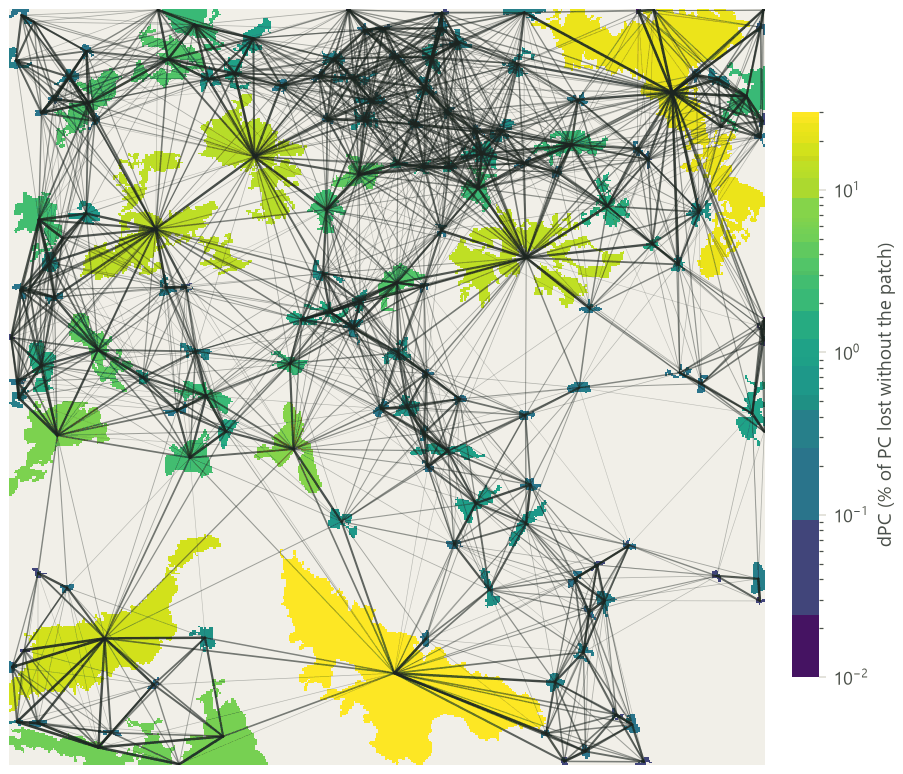
The last two nodes look ahead to part 3: conn.node_importance gives, for each patch, the share of PC lost if it were removed (dPC), and conn.to_map paints it on the patches. They are here because a map of where connectivity comes from helps to read the curve.

Read the results#

The dashboard: connectivity against distance#

Move the slider: each frame is a real run at one distance, the patches coloured by their dPC (the same scale for every frame) and the links drawn with their probability (darker: likelier). The numbers are those of conn.overall at that distance; the chart shows EC(PC) and EC(IIC) as a share of the forest's 51,569 ha.

Dispersal distance (probability 0.5) 250 m — The forest network for species that cross 250 m to 10 km with a probability of one half. Colours: the share of PC lost without each patch (dPC, logarithmic, from 0.01% to 30%). As the distance grows, the north fuses into one network and the large southern forests join it; EC(PC) climbs from 29% to 78% of the forest.

Dispersal distance (probability 0.5) 500 m — The forest network for species that cross 250 m to 10 km with a probability of one half. Colours: the share of PC lost without each patch (dPC, logarithmic, from 0.01% to 30%). As the distance grows, the north fuses into one network and the large southern forests join it; EC(PC) climbs from 29% to 78% of the forest.

What the curve says:

At short distances, ECA is the largest patches. At 250 m, EC(PC) is 14,751 ha, barely more than the 13,836 ha the patches would be worth with no movement at all (\(\sqrt{\sum a_i^2}\)). For a species that crosses little open land, this forest is a set of islands, and its connectivity is the size of its biggest islands.
The steep part of the curve is between 1 and 5 km. EC(PC) doubles, from 35% to 64% of the forest. This is the range of distances where the forest's connectivity is decided, and where the species that matter for planning live: a change of the landscape will change their reachable habitat the most.
It never reaches 100%. Even at 10 km, a disperser leaving one end of the map reaches the other with a low probability, so ECA stays below the habitat area. Only a "perfect" disperser would see all 51,569 ha as one.
EC(IIC) lies below EC(PC), because IIC ignores every pair farther apart than the threshold, while PC still gives them a small probability: the many weak, long moves add up.

The three fractions#

PC's numerator split into its intra, direct and step fractions (conn.overall's PCintra(%), PCdirect(%) and PCstep(%)). Stepping stones matter most between 3 and 7.5 km, where 40% of the reachable habitat is reached through other patches.

At 100 m, 95% of the reachable habitat is inside the patches themselves. By 2 km the three fractions are equal, and between 3 and 7.5 km the step fraction is the largest: for those species, two fifths of the reachable forest is reached only by hopping through woods in between. At still longer distances direct moves take over, because a species that crosses 20 km does not need stepping stones. The practical reading: for species of the middle range, the small woods that relay movement matter as much as the large forests. Which ones, the next part tells.

In the literature: how to report ECA

Report the habitat definition and its area, the distance measure, the dispersal distance(s) and the probability at them, ECA in hectares and as a share of the habitat, and, when comparing dates or scenarios, the change of ECA beside the change of habitat area. Saura et al. (2011) is a good model of this; Makurhini (Godínez-Gómez et al., 2026) and Conefor (Saura & Torné, 2009) compute the same numbers, so readers can reproduce them with either.

Settings that change the answer#

The dispersal distance changes ECA by a factor of three over the range above. If your species' distance is uncertain, give ECA at two or three distances that bracket it, as a curve or a short table.
The probability at that distance. A distance of 1 km at \(p = 0.5\) and a distance of 2 km at \(p = 0.25\) are the same kernel (\(0.5^{d/1000}\)). What matters is the kernel, not how you name it; say both numbers.
pij_min. Probabilities below it (0.01 by default) are treated as no link. At large distances this cuts many weak links and speeds the computation, with little effect on ECA; set it to 0 to keep every pair, as Conefor does.
Edge or centroid distances: centroids make every pair farther and lower ECA, the more so the larger the patches.
The patch attribute. Area is the default; a patch's habitat quality times its area (attribute and weighted = true in conn.graph_from_raster) makes ECA an amount of quality-weighted reachable habitat.
The study area changes PC and IIC (they divide by \(A_L^2\)) but not ECA or the fractions. Compare PC only between study areas of the same size; compare ECA freely.

Common pitfalls#

Comparing PC between regions of different size. Use ECA, or ECA over the habitat area.
Reading a high ECA as "well connected" without the habitat area. A large forest with poor connectivity can have a higher ECA than a small, perfectly connected one. Report both, and ECA over the area.
Forgetting the units. ECA is in the units of the attribute (here hectares). If the attribute is a quality index, ECA is in "quality units" and must be explained.
Patches cut by the border. As in part 1, patches cut by the edge of the study area count as smaller than they are, and their links outside are lost. The transboundary options of ProtConn (part 6) deal with this for reserves.
A single number for many species. A landscape well connected for a deer can be fragmented for a beetle. Report the distances, never "the connectivity" alone.

Going further#

Part 3: the importance of each patch: dPC and its intra, flux and connector fractions, link importance, and centralities.
Part 4: least-cost links: the same indices with distances through a resistance.
conn.eca_change and conn.eca_change_grid for changes between dates, and conn.connectivity_grid for connectivity mapped in hexagons over a region.
The operators: conn.overall, conn.graph, conn.graph_from_raster, conn.node_importance, conn.read_conefor, conn.write_conefor.

References#

Godínez-Gómez, O., Correa-Ayram, C., Goicolea, T., & Saura, S. (2026). Makurhini: an R package for comprehensive analysis of landscape fragmentation and connectivity. Environmental Modelling & Software, 201, 106981. https://doi.org/10.1016/j.envsoft.2026.106981
Pascual-Hortal, L., & Saura, S. (2006). Comparison and development of new graph-based landscape connectivity indices: towards the priorization of habitat patches and corridors for conservation. Landscape Ecology, 21(7), 959–967. https://doi.org/10.1007/s10980-006-0013-z
Saura, S., & Pascual-Hortal, L. (2007). A new habitat availability index to integrate connectivity in landscape conservation planning: comparison with existing indices and application to a case study. Landscape and Urban Planning, 83(2–3), 91–103. https://doi.org/10.1016/j.landurbplan.2007.03.005
Saura, S., & Rubio, L. (2010). A common currency for the different ways in which patches and links can contribute to habitat availability and connectivity in the landscape. Ecography, 33(3), 523–537. https://doi.org/10.1111/j.1600-0587.2009.05760.x
Saura, S., & Torné, J. (2009). Conefor Sensinode 2.2: a software package for quantifying the importance of habitat patches for landscape connectivity. Environmental Modelling & Software, 24(1), 135–139. https://doi.org/10.1016/j.envsoft.2008.05.005
Saura, S., Estreguil, C., Mouton, C., & Rodríguez-Freire, M. (2011). Network analysis to assess landscape connectivity trends: application to European forests (1990–2000). Ecological Indicators, 11(2), 407–416. https://doi.org/10.1016/j.ecolind.2010.06.011
Saura, S., Bastin, L., Battistella, L., Mandrici, A., & Dubois, G. (2017). Protected areas in the world's ecoregions: how well connected are they? Ecological Indicators, 76, 144–158. https://doi.org/10.1016/j.ecolind.2016.12.047