Suitability from logistic regressions

In CLUE-S every land use competes for every cell with a suitability: a number from 0 to 1 that says how likely the land use is in that cell, given what the cell is like. In this part you will make those suitability maps for the Plum Island Ecosystems with two nodes, a logistic regression (glm.fit) and its prediction (glm.predict); learn to read the coefficients as ecological statements ("built land is less likely on steep slopes"); and check, with a ROC curve, whether the maps really point at the places where land changed. You will also see a trap that catches many published models: a driver that explains the map perfectly and the change hardly at all.

The idea#

From presence to probability#

Ecologists know the logic from species distribution models. Take one class, say built land. Every cell of the map either is built (1) or is not (0). A logistic regression relates that presence to the cell's drivers (explanatory variables: elevation, slope, distance to the nearest town...) through a straight line on the scale of the log-odds:

Key idea: the logistic regression of a class

\[ \log \frac{p_i}{1 - p_i} = \beta_0 + \beta_1 x_{1,i} + \beta_2 x_{2,i} + \dots + \beta_k x_{k,i} \qquad\Longleftrightarrow\qquad p_i = \frac{1}{1 + e^{-(\beta_0 + \beta_1 x_{1,i} + \dots + \beta_k x_{k,i})}} \]

$ p_i $ is the probability that cell $i$ holds the class: its suitability;
$ x_{1,i} \dots x_{k,i} $ are the values of the $k$ drivers in cell $i$;
$ \beta_0 $ is the intercept, $ \beta_1 \dots \beta_k $ the coefficients, estimated from the map by maximum likelihood;
$ p / (1 - p) $ is the odds: a coefficient $ \beta $ multiplies the odds by $ e^{\beta} $ for each unit of its driver.

The regression is fitted on the cells of one map (lulcc fits it on the map the simulation starts from), and the fitted line is then evaluated in every cell to give a map of $ p $: the suitability map. CLUE-S fits one regression per class, each with its own drivers. Verburg et al. (2002) used exactly this for Sibuyan Island; lulcc (Moulds et al., 2015) and Terraflux fit it with R's glm algorithm (Terraflux reproduces R's glm.fit operation for operation, so the coefficients match R's).

What a suitability is, and what it is not#

The suitability of a class is where the class is, given the drivers, not where it will appear. These are different questions. A class that has been in place for centuries (the old town centres) and a class that spreads now (new suburbs) can sit on different land. The regression of the current map mixes both. Two consequences follow, and both will appear in the numbers below:

the best fit to the current map is not necessarily the best guide to future change;
a driver derived from the class itself (the distance to built land, for built land) fits the current map almost by definition.

An alternative is to fit the regression on the change itself (where the class appeared in an observed period): that is what PLUS's land expansion analysis does (see PLUS).

The classes are fitted separately

Each class has its own regression, so the suitabilities of a cell need not add up to 1: at Plum Island their sum ranges from 0.59 to 1.60 (1^st and 99^th percentiles). CLUE-S compares them across classes anyway; the iteration variables of part 1 shift each class up or down until the areas are right.

When to use it#

A logistic regression is the classic potential of CLUE-S and the default of terraflux new clue. It is a good choice when:

you have a few drivers with a clear meaning (terrain, accessibility, soils) and want coefficients you can report and defend;
the response to each driver is roughly monotonic (always rising or always falling);
you want a model that others can reproduce exactly, in R or in Terraflux.

Consider something else when the responses have thresholds or interactions that a straight line on the log-odds cannot follow (random forests, as PLUS uses: PLUS), when the change is driven by transitions rather than by classes (weights of evidence, in the first half of this category), or when a class's suitability is known from expert knowledge (give it as a map: any stack with a layer per class works as the suitability of lulcc.step).

What you need#

The map the regressions are fitted on: the land use at the start of the simulation, with class codes. Here, pie_landuse.tif, band 1985.
The drivers, a stack on the same grid, each layer named. Here, pie_drivers.tif: elevation, slope and dist_built_1985 (the distance to the built land of 1985, in metres). Download both from part 1.

The three drivers of Plum Island — The drivers of lulcc's Plum Island example: elevation, slope and the distance to the built land of 1985.

The drivers are weakly correlated with each other (elevation and slope: 0.30; the distance to built land and the others: below 0.1 in absolute value), so each coefficient can be read on its own. Check this for your own drivers: two strongly correlated drivers (two distances to roads of different kinds, say) share their effect and their coefficients become unstable.

Build the model#

Step 1: read the map and the drivers#

In the application, add a raster.read node for each file (library: IO), or declare them as the model's inputs. As a file, the model starts like this:

[inputs.start]
kind = "map"
path = "pie_landuse.tif"
band = "1985"          # a band by its name (or a 0-based index)

[inputs.drivers]
kind = "stack"
path = "pie_drivers.tif"

A map input reads one band; a stack input reads all the bands, named by their descriptions in the file. The regressions find the drivers by these names.

Step 2: fit the regressions (`glm.fit`)#

Add a glm.fit node (library: Land change simulation → lulcc and CLUE-S). Drag from $start to its landscape port and from $drivers to its drivers port. Its one setting that matters is formulas: the drivers of each class's regression. lulcc's vignette uses elevation and slope for forest and other land, and adds the distance to built land for built land:

The regressions of lulcc's vignette: a logistic regression per class, each with its own drivers.

Model file (TOML)

format = "terraflux/1"

[inputs.start]
kind = "map"
path = "pie_landuse.tif"
band = "1985"

[inputs.drivers]
kind = "stack"
path = "pie_drivers.tif"

[[nodes]]
id = "regression"
op = "glm.fit"
inputs = { landscape = "$start", drivers = "$drivers" }
params = { formulas = { 1 = ["elevation", "slope"], 2 = ["elevation", "slope", "dist_built_1985"], 3 = ["elevation", "slope"] } }
note = "Logistic regression of the presence of each class on its drivers (lulcc's glmModels)."

Without formulas, every class present in the map gets a regression on every driver. The intercept is always in. Two more settings, maxit (25) and epsilon (1e-8), are R's iteration limit and convergence tolerance; leave them.

Which cells take part? Every cell with a class in the map and a value in all the drivers of that class's regression (R's na.omit). Here that is 113,563 cells for each class.

Step 3: predict the suitability (`glm.predict`)#

Add a glm.predict node. Connect regression.model to model, the drivers to drivers, and the start map to landscape (optional: it keeps no-data cells as no data). Its output, suitability, is a stack with a layer per class, named by the class code: exactly what lulcc.step wants.

Two nodes give the suitability of every class in every cell.

Model file (TOML)

format = "terraflux/1"

[inputs.start]
kind = "map"
path = "pie_landuse.tif"
band = "1985"

[inputs.drivers]
kind = "stack"
path = "pie_drivers.tif"

[[nodes]]
id = "regression"
op = "glm.fit"
inputs = { landscape = "$start", drivers = "$drivers" }
params = { formulas = { 1 = ["elevation", "slope"], 2 = ["elevation", "slope", "dist_built_1985"], 3 = ["elevation", "slope"] } }

[[nodes]]
id = "suitability"
op = "glm.predict"
inputs = { model = "regression.model", drivers = "$drivers", landscape = "$start" }
note = "The suitability of each class at every cell, a layer per class."

[outputs.model]
from = "regression.model"

[outputs.suitability]
from = "suitability.suitability"

Why two nodes and not one? Because the fit and the prediction may use different drivers. The fit uses the drivers as they were on the fitting map; the prediction can use drivers that have changed since: a new road, or a distance to built land recomputed from the simulated map at every step. That is the subject of Dynamic drivers, where glm.predict moves inside the loop and glm.fit stays outside.

In the application

Select the suitability node and press Ctrl+Enter to run the model up to it, then look at its stack, a layer per class. To keep the coefficients, make regression.model an output of the model: a run writes it as model.json.

From the command line, the two outputs above are written by terraflux run: output/model.json (the coefficients) and output/suitability.tif (a band per class).

terraflux run suitability.toml
  wrote output\model.json
  wrote output\suitability.tif

Coefficients from elsewhere: `glm.coefficients`#

If the regressions were fitted elsewhere (in R, or in a published study), glm.coefficients gives them to the model directly, in the same form as model.json: per class, the drivers, the coefficients (intercept first), and R's pivot and rank (for a full-rank model, 1, 2, 3... and the number of coefficients). Here are Plum Island's built-land coefficients, as fitted above:

A regression given by its coefficients instead of fitted: the same suitability as before for built land.

Model file (TOML)

format = "terraflux/1"

[inputs.drivers]
kind = "stack"
path = "pie_drivers.tif"

[[nodes]]
id = "given"
op = "glm.coefficients"
params = { fits = [ { class = 2, drivers = ["elevation", "slope", "dist_built_1985"], coefficients = [1.63533, 0.00823, -0.04404, -0.02286], pivot = [1, 2, 3, 4], rank = 4 } ] }

[[nodes]]
id = "suitability"
op = "glm.predict"
inputs = { model = "given.model", drivers = "$drivers" }

Read the results#

The coefficients#

The regressions of lulcc's vignette on the map of 1985 (real fit, output/model.json):

Class	Intercept	elevation	slope	dist_built_1985 (per m)	Pseudo R²
Forest	−1.390	+0.0237	+0.0501		0.042
Built	+1.635	+0.0082	−0.0440	−0.02286	0.498
Other	+0.537	−0.0518	−0.0070		0.102

Read them as statements about the landscape:

Forest is more likely on higher and steeper land (both coefficients positive): the land least useful for building and farming kept its forest. But the pseudo R² of 0.04 says that elevation and slope explain very little of where forest is.
Built land falls off steeply with the distance to the built land of 1985: each 100 m multiplies the odds by $ e^{-0.02286 \times 100} = 0.10 $. It also avoids steep slopes (each unit of slope multiplies the odds by 0.96).
Other land is on low land (−0.052 per unit of elevation): along the coast, the marshes and the river valleys.

The pseudo R² here is McFadden's: $ 1 - D / D_0 $, where $D$ is the model's deviance and $D_0$ the deviance of a model with the intercept only (both are in model.json as deviance and null_deviance). It is not the R² of a linear regression: values of 0.2 to 0.4 are usually considered a good fit.

A response curve shows the same thing as a picture: the probability of built land along each driver, the other two held at their medians (computed from the fitted coefficients).

Response curves of built land — The probability of built land along each driver, from the fitted coefficients, the other drivers at their medians (elevation 34, slope 4.4, distance 141 m).

The suitability maps#

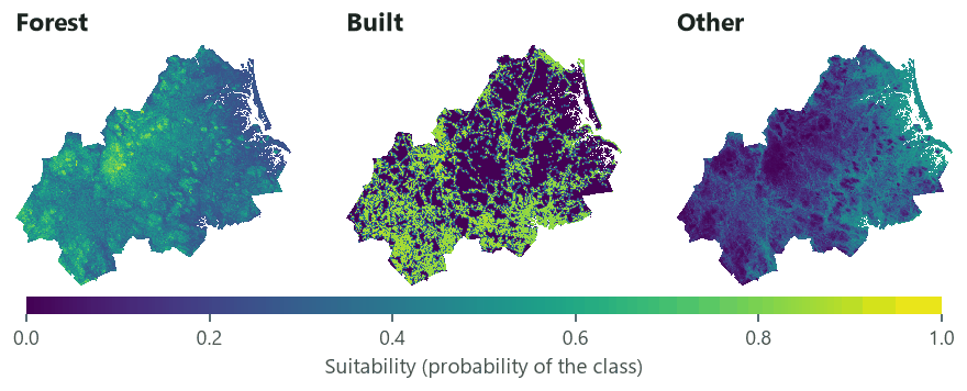
Suitability of the three classes — The suitability of forest, built and other land in 1985 (glm.predict). Built land's suitability is a network of high values around the built land of 1985.

Forest's and other land's suitabilities are smooth surfaces that follow the terrain, with values between 0.2 and 0.6 almost everywhere: they barely tell cells apart. Built land's map is sharp: close to 1 on and next to the built land of 1985, close to 0 a few hundred metres away. In the competition of CLUE-S, this means that built land will win the cells next to existing built land, and forest and other land will share the rest according to small differences of elevation.

Does the suitability point at the change? The ROC#

A suitability map is a ranking of the cells. The ROC (relative operating characteristic) asks how well the ranking separates the cells that hold (or gain) a class from those that do not: rank the cells from the most to the least suitable, and plot, for every threshold, the share of the class's cells above it (hits) against the share of the other cells above it (false alarms). The area under the curve (AUC) is 1 for a perfect ranking and 0.5 for a random one (Pontius & Schneider, 2001; Pontius & Parmentier, 2014).

ROC curves of the suitability maps (computed from the real outputs). Against the map they were fitted on, built land's suitability is nearly perfect; against the built land that appeared between 1985 and 1999, among the cells not built in 1985, it is barely better than chance.

The curves tell a story that every land change modeller should know:

Against the 1985 map, built land's suitability reaches an AUC of 0.94. This is circular: the distance to the built land of 1985 is 0 on every built cell of 1985, so the regression has learnt that built cells are built.
Against the new built land of 1985–1999 (among the cells that were not built in 1985), the AUC falls to 0.63. The suitability ranks the cells where change happened only a little better than chance.

The second number is the one that matters for a simulation. Report it, not the first. Pontius and Schneider (2001) introduced the ROC to land change modelling precisely to measure how well a suitability map points at the observed change, on the Ipswich watershed, in the same region of Massachusetts as these data.

Settings that change the answer#

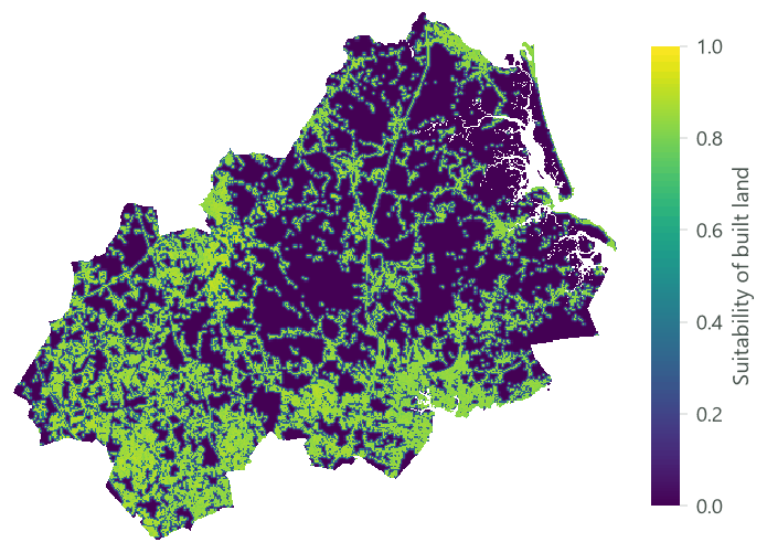
The drivers you choose change the suitability far more than any setting of the fit. The dashboard below is built from three real runs of glm.fit and glm.predict, with built land's regression on one, two and three drivers.

Drivers of built land 1 — Built land's suitability with one, two and three drivers (real runs). Elevation and slope alone give an almost flat map that ranks the cells little better than chance. Adding the distance to built land gives the sharp map of the vignette: a near-perfect fit to the map of 1985, and only a modest gain for the new built land.

Drivers of built land 2 — Built land's suitability with one, two and three drivers (real runs). Elevation and slope alone give an almost flat map that ranks the cells little better than chance. Adding the distance to built land gives the sharp map of the vignette: a near-perfect fit to the map of 1985, and only a modest gain for the new built land.

What to take from it:

Accessibility drivers matter most for built land. Without a distance to existing built land (or to roads, or to town centres), terrain alone says almost nothing about where people build at Plum Island.
A better fit to the map is not a better prediction of change. The pseudo R² jumps from 0.004 to 0.50; the AUC of the new built land only from 0.56 to 0.63.
Static distances age. The distance to the built land of 1985 is right in 1985 and wrong by 1999, when new suburbs have appeared. Recomputing it from the simulated map at every step is the job of Dynamic drivers.

Common pitfalls#

A driver missing where the class is. A cell missing any driver of a class gets no suitability for that class (NaN) and can never take it. Fill the gaps of the drivers, or crop the study area to where all of them exist.
Driver names that do not match. The formulas find the drivers by name: dist_built_1985 must be the name of a band of the stack (the error lists the names it found). Name the bands of your stack, or build it with stack.of from separate maps (each input's name becomes a layer's name).
Circular drivers. A distance to the class itself, a neighbourhood share of the class, a density of the class: they fit the current map by construction. Judge them on the change, with a ROC of the new cells.
Categorical drivers coded as numbers. A soil map with codes 1, 2, 3 is not a quantity: the regression would treat soil 3 as "more" than soil 1. Make a 0/1 layer per category (with raster.calc: soil == 2).
Reading coefficients of correlated drivers. When two drivers carry the same information, their coefficients can take opposite signs and still give the same suitability. Check correlations first.

Going further#

Part 3: The demand: how much of each class.
Part 4: A complete CLUE-S model, where these suitabilities compete.
Dynamic drivers: the distance to built land recomputed every year.
The weights of evidence, the other classic potential: see the first half of this category.
Reference: glm.fit, glm.predict, glm.coefficients.

References#

Moulds, S., Buytaert, W., & Mijic, A. (2015). An open and extensible framework for spatially explicit land use change modelling: the lulcc R package. Geoscientific Model Development, 8(10), 3215–3229. https://doi.org/10.5194/gmd-8-3215-2015
Pontius, R. G., Jr., & Parmentier, B. (2014). Recommendations for using the relative operating characteristic (ROC). Landscape Ecology, 29(3), 367–382. https://doi.org/10.1007/s10980-013-9984-8
Pontius, R. G., Jr., & Schneider, L. C. (2001). Land-cover change model validation by an ROC method for the Ipswich watershed, Massachusetts, USA. Agriculture, Ecosystems & Environment, 85(1–3), 239–248. https://doi.org/10.1016/S0167-8809(01)00187-6
Verburg, P. H., Soepboer, W., Veldkamp, A., Limpiada, R., Espaldon, V., & Mastura, S. S. A. (2002). Modeling the spatial dynamics of regional land use: the CLUE-S model. Environmental Management, 30(3), 391–405. https://doi.org/10.1007/s00267-002-2630-x

The idea#

From presence to probability#

What a suitability is, and what it is not#

When to use it#

What you need#

Build the model#

Step 1: read the map and the drivers#

Step 2: fit the regressions (glm.fit)#

Step 3: predict the suitability (glm.predict)#

Coefficients from elsewhere: glm.coefficients#

Read the results#

The coefficients#

The suitability maps#

Does the suitability point at the change? The ROC#

Settings that change the answer#

Common pitfalls#

Going further#

References#

Step 2: fit the regressions (`glm.fit`)#

Step 3: predict the suitability (`glm.predict`)#

Coefficients from elsewhere: `glm.coefficients`#