

Ecosystem services with InVEST, part 7 of 8
Seasonal water yield
InVEST's seasonal water yield model in Terraflux - the quickflow of each month from the curve number, the local recharge and the water cells take from upslope, the baseflow that reaches the streams, the alpha, beta and gamma parameters, and what a land use scenario does to the wet and the dry season.
- Level
- Advanced
- Time
- 60 min
- 11. The ideas
- 22. Carbon
- 33. Habitat quality
- 44. Water yield
- 55. Sediment
- 66. Nutrients
- 77. Seasonal water
- 88. Pollination
A town that takes its water from a stream cares less about how much water the stream carries in a year than about how much it carries at the end of the dry season. In southeastern Brazil, where most of the rain falls between October and March, that dry-season water is baseflow: rain that soaked into the soil months before and seeps slowly to the stream. The rest of the streamflow is quickflow, the water that runs off during and just after a storm. Land use changes both. In this tutorial you will build InVEST's seasonal water yield model in Terraflux on Ribeirão Claro, read its maps of quickflow, recharge and baseflow and the monthly table of the two watersheds, see which parameters change the answer, and compare the scenario of 2040 with 2020. At the end you will know what the model's indices mean, and why InVEST's guide says to read them as relative values, not as volumes.
The idea#
The annual water yield model (part 4) answers how much of the year's rain leaves a watershed. It cannot say when. The seasonal model splits the water by how fast it moves:
- quickflow (QF) has a residence time in the watershed of hours to days: runoff over the surface and fast flow just below it, during and soon after the rain;
- baseflow has a residence time of months to years: rain that infiltrates, recharges the soil and the groundwater, and reaches the streams in dry weather.
In a seasonal climate, the guide that comes with InVEST notes, the baseflow is likely worth more than the quickflow unless there is a large reservoir to store the storms' water (Natural Capital Alliance, 2026). Brauman et al. (2007) made a related point for hydrologic services in general: what they are worth depends on the quantity of water, but also on its quality, its location and its timing.
The model computes three indices for every cell, from monthly climate, the land use, the soils and the elevation: the quickflow, the local recharge, and the baseflow. Its quickflow comes from Guswa et al. (2018); Hamel et al. (2020a) describe the model and test it in two large basins.
Quickflow: the curve number, month by month#
The curve number (CN) method was developed by the US Soil Conservation Service (now the Natural Resources Conservation Service, NRCS) to predict the runoff of a single storm from the rain, the soil and the cover (USDA-NRCS, 2004b; its history and limits are reviewed by Ponce & Hawkins, 1996). The soil enters through its hydrologic soil group: A (sands and deep, well-drained soils, which take water fast) to D (clays, shallow soils and soils with a high water table, which take little) (USDA-NRCS, 2009). The cover enters through a table of curve numbers, one per class and soil group (USDA-NRCS, 2004a), from about 30 (forest in good condition on group A) to 98 (pavement).
Key idea: from one storm to a month of storms
For one storm of \(p\) inches, the curve number method gives the runoff
where \(S\) (inches) is the maximum potential retention, the water the soil and the cover can still take in, and \(0.2\,S\) the rain held before any runoff starts. A CN of 100 gives \(S = 0\) (everything runs off); a CN of 50 gives \(S = 10\) inches.
Monthly data say how much it rained, not how the rain was split into storms. Guswa et al. (2018) assumed that the depths of the rainy days of a month follow an exponential distribution with mean \(a_{i,m} = P_{i,m} / n_m\) (converted to inches), and integrated the storm equation over it. The quickflow of cell \(i\) in month \(m\) is then
with \(P_{i,m}\) the rain of the month (mm), \(n_m\) the number of rain events in the month (days with more than 0.1 mm), \(S_i\) from the cell's curve number (its class and soil group), \(E_1\) the exponential integral, and 25.4 the millimetres of an inch. On the stream cells the quickflow is the rain itself. The annual quickflow \(\text{QF}_i\) is the sum of the twelve months.

A worked cell: pasture on a group C soil, CN 79, so \(S = 1000/79 - 10 = 2.66\) inches (67.5 mm). In January it rains 260 mm in 18 events, a mean of \(a = 14.4\) mm per event: \(S/a = 4.67\) and the equation gives 27.8 mm of quickflow, 11% of the rain. In July, 35 mm in 3 events (11.7 mm each), it gives 2.6 mm. The same 260 mm of January in 9 events of 28.9 mm would give 67.0 mm. The same January on a group A soil (CN 49) gives 0.6 mm; on a group D soil (CN 84), 44.8 mm.
Local recharge, and the water from upslope#
What does not run off quickly either evaporates or recharges the soil. The model writes the water balance of each cell over the year from twelve monthly balances, and lets a cell evaporate, in a dry month, part of the water that the cells above it recharged.
Key idea: local recharge
- \(L_i\), the local recharge of cell \(i\) (mm per year). It is negative where the cell evaporates more than its own rain leaves it, using water from upslope (the guide calls it an "upslope subsidy");
- \(\text{AET}_{i,m}\), the actual evapotranspiration of the month: the potential evapotranspiration \(\text{PET}\) (the reference evapotranspiration \(\text{ET}_0\) of the climate times the crop coefficient \(K_c\) of the class in that month), unless the water runs short;
- \(L_{\text{sum.avail},i}\), the recharge available from upslope: the sum, over the cells \(j\) that drain into \(i\), of \(p_{ji}\,(L_{\text{avail},j} + L_{\text{sum.avail},j})\), \(p_{ji}\) being the share of \(j\)'s flow that goes to \(i\);
- \(L_{\text{avail},i} = \min(\gamma\,L_i,\; L_i)\), the part of a cell's recharge that the cells below can use (all of it if negative);
- \(\alpha_m\), the share of the upslope recharge available in month \(m\) (default \(1/12\): the soil spreads it evenly over the year); \(\beta\), the share of that subsidy a cell may evaporate (default 1); \(\gamma\), the share of a cell's recharge passed on to the cells below (default 1).
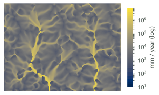
\(L_{\text{sum.avail}}\) is a sum of depths over all the cells upslope, not a mean, so it grows along the flow paths: here from 0 on the ridges to millions of millimetres on the main rivers. That is why, as you will see, even a small \(\beta\) lets the cells near the streams meet their evaporative demand.
Baseflow: what reaches the stream#
A cell's recharge is only potential baseflow: on its way down, part of it may be evaporated by the cells below. The model follows each path from the streams up.
Key idea: baseflow
where the sum runs over the cells \(j\) that \(i\) drains into, \(L_{\text{sum},i}\) is the recharge of the cell and of all the cells upslope (routed by the same shares \(p\)), \(B_{\text{sum},i}\) the baseflow through the cell, and \(B_i\) the baseflow index of the cell: its contribution to the slow flow that reaches a stream.
Two numbers summarise each watershed: \(Q_b\) (qb), the mean local recharge of its cells, and the sum of
\(V_{R,i} = L_i / \sum_k L_k\) (vri_sum), its share of the recharge of the whole area.
With the default \(\gamma = 1\), \(L_{\text{avail},j} = L_j\) and the term in the bracket reduces to \(B_{\text{sum},j} / L_{\text{sum},j}\); since that ratio is 1 at the streams, it is 1 everywhere, and \(B_i\) is simply \(\max(L_i, 0)\). The runs below confirm it: with the defaults, Terraflux's baseflow equals the positive part of the local recharge in every cell. The routing of the baseflow only matters when \(\gamma < 1\) (see Settings).
Terraflux and InVEST
The operator is InVEST 3.20's model as landschaft computes it, in InVEST's types and with its expressions; Terraflux's tests compare its maps and tables with landschaft's to the bit. landschaft is tested cell by cell against natcap.invest 3.20.2 with four of its bugs corrected: InVEST takes the mean of the upslope terms of \(L_{\text{sum.avail}}\) instead of their sum by the shares of the flow (eq. 103 of its guide), gives \(B_{\text{sum}} = 0\) to cells that drain off the edge of the raster, computes a recharge for cells without elevation that a D8 direction points into, and truncates fractional curve numbers when the land use and soil maps hold integers. Against InVEST as released, the curve numbers, the streams, the quickflow and the annual precipitation are the same to the bit; \(L_{\text{sum.avail}}\), and so AET, \(L\) and \(B\), differ where several cells drain into one.
When to use it#
- Where to protect or restore for the dry season: the parcels whose recharge feeds the streams (the baseflow index), for a water fund or payments for watershed services upstream of an intake.
- Scenarios: whether clearing forest, planting eucalyptus or expanding a town gives more storm runoff, less dry-season flow, or both.
- The month-to-month split of the streamflow between quickflow and baseflow, to compare with a gauge.
Hamel et al. (2020a) applied it in two large basins, in Peru and Myanmar, and compared it with observed flows and other models: the spatial pattern of the baseflow contributions correlated well with that of an established model in Peru (\(r^2 = 0.81\) at the parcel scale), and in Myanmar the model represented the month-to-month variation of the flow satisfactorily (Nash-Sutcliffe efficiency 0.6 to 0.8), with errors that depended on the scale. In the watershed program of Camboriú, in Santa Catarina, Hamel et al. (2020b) found that hydrologic modelling and monitoring gave the program scientific credibility, but that the detailed design of the program did not use it: decide first which decision the model must inform.
The annual model or the seasonal one? Use the annual model (services.water_yield) for the total water
of a year, and for hydropower and consumption, which it values. Use the seasonal one when the timing matters,
and when you want to see the trade-off the annual model cannot: a forest evaporates more (less water in a
year) but may let more rain soak in (more water in the dry season). The two do not compute the same thing: the
annual model has no routing and no quickflow, the seasonal one no valuation.
What it is not. The guide is explicit that the equations are extremely simplified in space and time, that
the absolute numbers are very uncertain, and that the indices should be read as relative values across the
landscape, not as volumes (Natural Capital Alliance, 2026). The baseflow is computed for the year; the
monthly table spreads it evenly over the twelve months. There is no snow, no groundwater storage from one year to
the next, no channel, and the quickflow ignores the slope. For daily flows, floods, groundwater and a calibrated
water balance, use a process model such as SWAT+ (swat.run; see the
SWAT+ tutorial), which needs much more data.
What you need#
Every raster on the grid of the DEM (the same rows, columns and cells), projected in metres:
| Input | File | Unit |
|---|---|---|
dem |
dem.tif |
m; the model fills its depressions and routes the flow over it |
lulc |
lulc_2020.tif |
class codes |
soil_group |
soil_group.tif |
1 (A), 2 (B), 3 (C), 4 (D) |
precipitation |
precipitation_monthly.tif |
12 layers (January to December), mm per month |
et0 |
et0_monthly.tif |
12 layers, reference evapotranspiration, mm per month |
biophysical |
biophysical_swy.csv |
by class: lucode, cn_a to cn_d, kc_1 to kc_12 |
watersheds |
watersheds.gpkg |
polygons (with ws_id, else numbered 1, 2...) for the tables |
the setting rain_events |
twelve numbers: the rain events of each month |
A stack of twelve months can be a file of twelve bands, as here, or a folder of twelve files read as one stack
by raster.read (its layers in the order of the files' names: name them 01.tif to 12.tif). Instead of
one series of rain events for the whole area you can give a map of climate zones (climate_zones) and a
table (climate_zone_table: cz_id, jan ... dec), one series per zone; one or the other, not both.
The series' landscape has annual rasters of rain and ET0 but no months and no soil groups, so this tutorial makes them (illustrative): each month is the annual map times the share of that month in the climate of the interior of São Paulo or southern Minas Gerais, wet from October to March, dry from April to September. The soil groups follow the soil depth of part 4: deep soils on gentle ground are A or B, shallow soils on the steep slopes are C or D, and the wet soils along the rivers are D. Download seasonal-inputs.zip (0.2 MB) and unzip it into the folder of the series' files (ribeirao-claro.zip, which has the DEM, the land use maps and the watersheds).


The biophysical table. The curve numbers here are in the range of the USDA's tables (USDA-NRCS, 2004a) for woods in good and fair condition (forest, eucalyptus), pasture, row crops and residential land; use local values where they exist. The crop coefficients \(K_c\) (Allen et al., 1998) follow the seasons: the pasture dries in winter, the cropland is bare after the summer harvest.
| lucode | class | cn_a | cn_b | cn_c | cn_d |
|---|---|---|---|---|---|
| 1 | Forest | 30 | 55 | 70 | 77 |
| 2 | Pasture | 49 | 69 | 79 | 84 |
| 3 | Cropland | 65 | 75 | 82 | 86 |
| 4 | Eucalyptus | 36 | 60 | 73 | 79 |
| 5 | Urban | 77 | 85 | 90 | 92 |
| 6 | Water | 99 | 99 | 99 | 99 |
| class | kc_1 ... kc_12 (January to December) |
|---|---|
| Forest | 1.0 from October to April, 0.95 in May and September, 0.9 from June to August |
| Pasture | 0.85, 0.85, 0.85, 0.8, 0.7, 0.6, 0.55, 0.55, 0.6, 0.75, 0.85, 0.85 |
| Cropland | 1.1, 1.15, 0.9, 0.6, 0.5, 0.4, 0.35, 0.35, 0.4, 0.5, 0.7, 0.95 |
| Eucalyptus | 1.05 from October to March, 1.0 in April, May and September, 0.95 from June to August |
| Urban | 0.3 all year |
| Water | 1.0 all year |
Build the model#
Step 1: quickflow, recharge and baseflow#
- Add
raster.readnodes fordem.tif,lulc_2020.tif,soil_group.tif,precipitation_monthly.tifandet0_monthly.tif, atable.readforbiophysical_swy.csvand avector.readforwatersheds.gpkg. Rename each after its content. - Add
services.seasonal_water_yield(subject Ecosystem services) and drag from each reader's output port to the input of its name: the twelve-band files go toprecipitationandet0, which take a stack. - In the Node pane set
threshold, the number of cells that must drain into a cell for it to be a stream (required: here 1,000 cells, 90 ha, as in the sediment tutorial), andrain_events, the twelve numbers. Leavealpha,beta,gammaandmethodat InVEST's defaults (1/12, 1, 1,mfd). - Run (Ctrl+Enter).
Model file (TOML)
format = "terraflux/1"

[[nodes]]
id = "dem"
op = "raster.read"
params = { path = "dem.tif" }

[[nodes]]
id = "lulc"
op = "raster.read"
params = { path = "lulc_2020.tif" }

[[nodes]]
id = "soils"
op = "raster.read"
params = { path = "soil_group.tif" }

[[nodes]]
id = "precipitation"
op = "raster.read"
params = { path = "precipitation_monthly.tif" }
note = "12 bands, mm per month"

[[nodes]]
id = "et0"
op = "raster.read"
params = { path = "et0_monthly.tif" }
note = "12 bands, mm per month"

[[nodes]]
id = "biophysical"
op = "table.read"
params = { path = "biophysical_swy.csv" }
note = "lucode, cn_a ... cn_d, kc_1 ... kc_12."

[[nodes]]
id = "watersheds"
op = "vector.read"
params = { path = "watersheds.gpkg" }

[[nodes]]
id = "swy"
op = "services.seasonal_water_yield"
inputs = { dem = "dem.raster", lulc = "lulc.raster", soil_group = "soils.raster", precipitation = "precipitation.raster", et0 = "et0.raster", biophysical = "biophysical.table", watersheds = "watersheds.vector" }
params = { threshold = 1000, rain_events = [18, 15, 13, 7, 6, 4, 3, 3, 6, 10, 12, 16] }
Behind the node, as in InVEST: the DEM's depressions filled, the flow routed by multiple flow directions
(mfd, each cell's water shared among its lower neighbours) or d8 (all of it to the steepest), the streams
traced, the curve numbers looked up by class and soil group, the twelve months of quickflow, then the recharge
from the ridges down and the baseflow from the streams up. Its outputs:
| Output | What it is | Unit |
|---|---|---|
quickflow, quickflow_monthly |
QF of the year; of each month (a stack of 12 layers) | mm |
aet, annual_precipitation |
actual evapotranspiration and rain of the year | mm |
local_recharge |
\(L\) | mm |
l_avail, l_sum_avail, l_sum |
\(L_{\text{avail}}\), \(L_{\text{sum.avail}}\), \(L_{\text{sum}}\) (sums over the cells upslope) | mm |
baseflow, b_sum |
\(B\), \(B_{\text{sum}}\) | mm |
vri |
\(V_R\), the cell's share of the total recharge | |
stream |
the streams (1) | |
watershed_table |
by watershed: ws_id, qb, vri_sum, geom_id (the polygon's row, from 0) |
mm |
monthly_table |
by watershed and month: geom_id, month, quickflow, baseflow, precipitation |
m³ |
The node stops with a message on soil groups other than 1 to 4, land use classes missing from the table, stacks that do not hold twelve layers or rasters off the DEM's grid, a DEM in longitude and latitude, and rain events given together with climate zones (or neither).
A recharge map of your own
Connect a map of local recharge (mm) to recharge and leave out the land use, the table and the climate:
the node then only routes that recharge to the baseflow (local_recharge, l_avail, l_sum, baseflow,
b_sum, vri, stream and watershed_table), as InVEST's "user-defined local recharge" option does. Use it
with the recharge of another model.
Step 2: the tables and the months to files#
- Add two
table.writenodes and connectmonthly_tableandwatershed_tableto them. - Add a
raster.writeand connectquickflow_monthly; with{name}in its path it writes a file per layer, named by the month (1 to 12).
Model file (TOML)
format = "terraflux/1"

[[nodes]]
id = "swy"
op = "services.seasonal_water_yield"
inputs = { dem = "dem.raster", lulc = "lulc.raster", soil_group = "soils.raster", precipitation = "precipitation.raster", et0 = "et0.raster", biophysical = "biophysical.table", watersheds = "watersheds.vector" }
params = { threshold = 1000, rain_events = [18, 15, 13, 7, 6, 4, 3, 3, 6, 10, 12, 16] }

[[nodes]]
id = "months"
op = "table.write"
inputs = { table = "swy.monthly_table" }
params = { path = "monthly_2020.csv" }

[[nodes]]
id = "sheds"
op = "table.write"
inputs = { table = "swy.watershed_table" }
params = { path = "watersheds_2020.csv" }

[[nodes]]
id = "qf"
op = "raster.write"
inputs = { value = "swy.quickflow_monthly" }
params = { path = "quickflow/qf_{name}.tif" }
Read the results#
The maps of the year#


Over the landscape, of 1,512 mm of rain a year, 95 mm (6%) leave as quickflow, 980 mm evaporate and 436 mm recharge on average. Only 3% of the cells have a negative recharge: the 902 stream cells, and 395 cells off the streams (0.9% of them). Means by class:
| Class | Cells | Rain (mm) | Quickflow (mm) | AET (mm) | Recharge (mm) | Baseflow (mm) |
|---|---|---|---|---|---|---|
| Forest | 17,077 | 1,563 | 61 | 1,131 | 371 | 372 |
| Pasture | 15,501 | 1,470 | 59 | 904 | 506 | 506 |
| Cropland | 8,225 | 1,516 | 60 | 827 | 630 | 630 |
| Eucalyptus | 611 | 1,508 | 15 | 1,214 | 280 | 280 |
| Urban | 624 | 1,418 | 255 | 365 | 798 | 798 |
| Water | 260 | 1,410 | 1,160 | 1,222 | -972 | 0 |
As in the annual model, a class's numbers mix the class with where it grows. Forest has as little quickflow as pasture although its curve numbers are lower, because it grows on the steep slopes: 71% of its cells are on the shallow soils of groups C and D, against 16% of the pasture's. On one class, the soil group decides:
| Soil group | CN | Cells | Quickflow (mm) | Recharge (mm) |
|---|---|---|---|---|
| A | 49 | 1,253 | 3 | 592 |
| B | 69 | 11,817 | 48 | 533 |
| C | 79 | 1,735 | 121 | 360 |
| D | 84 | 696 | 197 | 270 |
The two maps of the routing, \(L_{\text{sum.avail}}\) and \(B_{\text{sum}}\), are sums over all the cells upslope, so they show the drainage network more than the cells (their unit is millimetres summed over cells: multiply by the area of a cell, 900 m², and divide by 1,000 to get m³):

The months#
The output quickflow_monthly holds a map per month, and monthly_table sums the quickflow, the baseflow and
the rain of each watershed in m³ (for the first polygon, geom_id 0, which is ws_id 1, from January to April:
403,149, 281,460, 204,663 and 70,882 m³ of quickflow, 618,473 m³ of baseflow each month). Divided by the area of
the two watersheds (3,065 ha), in millimetres:


The flat baseflow is not a prediction that the dry season flows as much as the wet one: the model has no store that carries the summer's recharge into the winter month by month. To compare with a gauge, the guide compares the observed flow with quickflow plus baseflow, and warns that the monthly split of the baseflow is crude (Natural Capital Alliance, 2026).
The watersheds#
| Watershed | Area (ha) | qb (mm) | vri_sum | Rain (mm) | Quickflow (mm) | Baseflow (mm) | Quickflow (Mm³) | Baseflow (Mm³) |
|---|---|---|---|---|---|---|---|---|
| 1 | 1,827 | 368.8 | 0.397 | 1,482 | 106 | 406 | 1.94 | 7.42 |
| 2 | 1,238 | 431.5 | 0.315 | 1,506 | 98 | 462 | 1.21 | 5.71 |
The baseflow of a watershed (406 mm in watershed 1) is larger than its mean recharge qb (369 mm): the cells
with a negative recharge, the streams above all, count 0 in the baseflow but count their deficit in qb. Report
which one you use.
Reporting a seasonal water yield analysis
Report the sources of the monthly rain and ET0 (the guide recommends that the ET0 be computed from the same rain data), the rain events and how you counted them, the soil groups, the table of curve numbers and \(K_c\), the threshold, \(\alpha\), \(\beta\), \(\gamma\) and the routing. Show the maps of quickflow and baseflow and the monthly table of each watershed for each scenario, and present them as relative contributions, as the guide advises, unless you have calibrated the model against measured flows.
The scenario of 2040#
Run the model again with lulc_2040.tif: forest edges cleared to pasture on gentle ground, pasture turned to
cropland, a larger town, a new plantation, and the pasture and crops along the rivers restored to forest.


| Quantity | 2020 | 2040 | Change |
|---|---|---|---|
| Quickflow (mm) | 102.8 | 118.7 | +15.5% |
| Baseflow (mm) | 428.6 | 458.3 | +6.9% |
| Quickflow, October to March (mm) | 84.9 | 98.3 | +15.8% |
| Evapotranspiration (mm), mean of the cells | 980.3 | 932.3 | -4.9% |
| Local recharge (mm), mean of the cells | 436.5 | 466.8 | +6.9% |
| 2020 to 2040 | Area (ha) | Quickflow (mm) | AET (mm) | Baseflow (mm) |
|---|---|---|---|---|
| Pasture to Cropland | 565 | 42.7 | -63.2 | 20.5 |
| Forest to Pasture | 532 | 72.1 | -259.9 | 187.5 |
| Forest to Cropland | 82 | 112 | -308.8 | 196.7 |
| Pasture to Forest | 61 | -102.5 | 271.3 | -154.3 |
| Cropland to Forest | 54 | -151.6 | 331.3 | -176.2 |
| Pasture to Urban | 33 | 174 | -550.7 | 376.6 |
| Cropland to Urban | 27 | 76 | -488.1 | 412 |
| Pasture to Eucalyptus | 19 | -39.1 | 315.1 | -276 |
| Forest to Urban | 13 | 337.4 | -812.3 | 474.9 |
| Forest to Eucalyptus | 9 | 16.6 | 54.6 | -71.2 |
In this model, clearing forest gives more water in both seasons: the evaporation it removes outweighs the rain it sends into quickflow. Whether that happens in a real watershed depends on what the clearing does to the soil. Bruijnzeel (2004), reviewing tropical forests, stressed that when the soil is compacted after clearing its infiltration falls, the extra rain leaves in the storms, and the dry-season flow can fall instead. The model sees the soil only through the curve number: to test that case, give the new pasture the curve numbers of a pasture in poor condition, or the next soil group, and run again. The unchanged cells keep their baseflow (a change of −0.004 mm on average): with \(\gamma = 1\) a cell's baseflow is the positive part of its own recharge, and the recharge of an unchanged cell hardly moves.
Settings that change the answer#
Beta: the water a cell may take from upslope#
\(\beta\) scales the upslope subsidy. At \(\beta = 0\) no cell evaporates water from upslope, and the recharge can never be negative. Because \(L_{\text{sum.avail}}\) grows so fast down the flow paths, a tiny \(\beta\) is already enough for most cells to meet their demand:


Most of the effect is between \(\beta = 0\) and \(\beta = 0.1\): above that, the landscape's recharge changes by
less than 10 mm. InVEST's guide describes \(\beta\) as a function of the local topography and soils (the storage
a cell has) and suggests, as an alternative to the default of 1, the topographic wetness index (Natural Capital
Alliance, 2026); in Terraflux beta is one number for the whole landscape.
Gamma: a warning#
\(\gamma\) is the share of a cell's recharge passed on to the cells below. On the evaporation and the recharge it acts almost exactly as \(\beta\) does (the same means here to 0.1 mm). On the baseflow it does something else:
| gamma | AET (mm) | Recharge (mm) | Baseflow (mm) |
|---|---|---|---|
| 0 | 891.9 | 524.9 | 4,126.9 |
| 0.25 | 977.9 | 438.9 | 1,533 |
| 0.5 | 979.9 | 436.9 | 895.5 |
| 0.75 | 980.2 | 436.6 | 615 |
| 1 | 980.3 | 436.5 | 464 |
This follows from the baseflow equation: with \(\gamma < 1\), \((1 - L_{\text{avail},j}/L_{\text{sum},j})/(L_{\text{sum},j} - L_j)\) is larger than \(1/L_{\text{sum},j}\) wherever \(L_j > 0\) (and the recharge upslope of \(j\) is positive), so the ratio \(B_{\text{sum}}/L_{\text{sum}}\) grows at every step up from the streams, and the baseflow of the cells far from a stream can exceed their recharge many times. Such values are not water. Keep \(\gamma = 1\) unless you have a reason and check that the baseflow stays below the recharge.
Alpha: when the upslope water is available#
The default \(\alpha_m = 1/12\) assumes the soil releases the upslope recharge evenly through the year. For highly
seasonal climates the guide suggests the share of the previous month's rain in the year's,
\(P_{m-1}/P_{\text{annual}}\) (Natural Capital Alliance, 2026). Give alpha as twelve numbers: here 0.153 for
January (the share of December's rain), 0.181, 0.139, 0.112, 0.049, 0.042, 0.031, 0.024, 0.021, 0.049, 0.087
and 0.112.
| alpha | AET (mm) | Recharge (mm) | Baseflow (mm) |
|---|---|---|---|
| 1/12 every month (default) | 980.3 | 436.5 | 464 |
| the previous month's share of the rain | 978.6 | 438.2 | 465.7 |
Here it hardly matters (2 mm), for the same reason as \(\beta\): the subsidy is so large that most cells meet
their demand in any month. It matters more where the upslope areas are small or the dry season long. alpha
also takes one number, or a fraction as text ("1/12").
The stream threshold#
Stream cells have a quickflow equal to the rain, so the threshold changes the quickflow directly:
Choose the threshold so that the streams match the real rivers on a map or on imagery (the streams and watersheds tutorial shows how), and use the same in every scenario.
Multiple flow directions or D8#
With method = "d8" the landscape's mean quickflow falls from 95 to 84 mm and the recharge rises from 436 to
454 mm: the two route the water differently and trace different streams. Report the routing, and keep it for
every scenario.
Common pitfalls#
- Annual maps instead of months.
precipitationandet0are twelve layers in mm per month; an annual map repeated twelve times gives twelve times the rain. - The order of the months. The layers are read in order: bands 1 to 12, or the files sorted by name
(
1.tif,10.tif,11.tif,12.tif,2.tif... is the wrong order: write01.tif). - Grids. Every raster must have the DEM's rows and columns; InVEST resamples them to the DEM, Terraflux
stops. Put them on the DEM's grid first with
raster.match. - Soil groups as letters or other codes. The map holds 1, 2, 3, 4; dual groups (A/D, B/D...) must be assigned to one group first.
- Curve numbers for the wrong condition. A pasture in poor condition has a higher CN than one in good condition; the choice can decide whether a scenario gains or loses dry-season water.
- Towns that recharge. With a \(K_c\) of 0.3 and a curve number of 77 to 92, the town evaporates little and sends little to quickflow, so the model credits it with the highest recharge of all (798 mm), and the growth of the town raises the baseflow in 2040. Paved surfaces, gutters and storm drains are not in the model: give urban classes higher curve numbers, or leave them out of the conclusions.
- Rain events. Count days with more than 0.1 mm of rain, as the guide defines an event; fewer, larger events give much more quickflow.
- Reading the indices as volumes. The guide asks you to read the quickflow, recharge and baseflow as relative contributions; summing millimetres over cells and multiplying by the area of the watershed gives volumes orders of magnitude too large. Use the monthly table, which sums the cells' volumes.
Going further#
- Annual water yield, part 4: the water of a year, its consumption and its value as hydropower.
- Sediment delivery ratio, part 5, and Nutrient delivery ratio, part 6: the same streams and the soil and nutrients they carry.
- Crop pollination by wild bees, part 8, the next part.
- Watershed simulation with SWAT+ for daily flows and a full water balance.
- Ecosystem service models: the ideas for the series as a whole.
- Monte Carlo uncertainty to carry the uncertainty of the curve numbers, \(K_c\) and \(\beta\) into the maps.
- The operators' reference:
services.seasonal_water_yield,services.water_yield,raster.match.
References#
- Allen, R. G., Pereira, L. S., Raes, D., & Smith, M. (1998). Crop evapotranspiration: Guidelines for computing crop water requirements (FAO Irrigation and Drainage Paper 56). Food and Agriculture Organization of the United Nations.
- Brauman, K. A., Daily, G. C., Duarte, T. K., & Mooney, H. A. (2007). The nature and value of ecosystem services: An overview highlighting hydrologic services. Annual Review of Environment and Resources, 32, 67–98. https://doi.org/10.1146/annurev.energy.32.031306.102758
- Bruijnzeel, L. A. (2004). Hydrological functions of tropical forests: Not seeing the soil for the trees? Agriculture, Ecosystems & Environment, 104(1), 185–228. https://doi.org/10.1016/j.agee.2004.01.015
- Guswa, A. J., Hamel, P., & Meyer, K. (2018). Curve number approach to estimate monthly and annual direct runoff. Journal of Hydrologic Engineering, 23(2), 04017060. https://doi.org/10.1061/(ASCE)HE.1943-5584.0001606
- Hamel, P., Valencia, J., Schmitt, R., Shrestha, M., Piman, T., Sharp, R. P., Francesconi, W., & Guswa, A. J. (2020a). Modeling seasonal water yield for landscape management: Applications in Peru and Myanmar. Journal of Environmental Management, 270, 110792. https://doi.org/10.1016/j.jenvman.2020.110792
- Hamel, P., Bremer, L. L., Ponette-González, A. G., Acosta, E., Fisher, J. R. B., Steele, B., Cavassani, A. T., Klemz, C., Blainski, E., & Brauman, K. A. (2020b). The value of hydrologic information for watershed management programs: The case of Camboriú, Brazil. Science of the Total Environment, 705, 135871. https://doi.org/10.1016/j.scitotenv.2019.135871
- Natural Capital Alliance. (2026). InVEST User's Guide (3.20): Seasonal water yield. https://storage.googleapis.com/releases.naturalcapitalproject.org/invest-userguide/latest/en/seasonal_water_yield.html
- Ponce, V. M., & Hawkins, R. H. (1996). Runoff curve number: Has it reached maturity? Journal of Hydrologic Engineering, 1(1), 11–19. https://doi.org/10.1061/(ASCE)1084-0699(1996)1:1(11)
- USDA-NRCS. (2004a). National Engineering Handbook, Part 630 Hydrology, Chapter 9: Hydrologic soil-cover complexes. U.S. Department of Agriculture, Natural Resources Conservation Service.
- USDA-NRCS. (2004b). National Engineering Handbook, Part 630 Hydrology, Chapter 10: Estimation of direct runoff from storm rainfall. U.S. Department of Agriculture, Natural Resources Conservation Service.
- USDA-NRCS. (2009). National Engineering Handbook, Part 630 Hydrology, Chapter 7: Hydrologic soil groups. U.S. Department of Agriculture, Natural Resources Conservation Service.