

Reclassify, calculate and save
Change a map's classes with rules, compute new maps cell by cell with map algebra, fill gaps, derive slope and hillshade from an elevation model, and save the results in the right file type.
- Level
- Beginner
- Time
- 35 min
Most analyses start by turning the maps you have into the maps a method needs: a land cover of 26 classes into
"forest" and "not forest", an elevation model into a slope, a map with holes into a complete one. In this tutorial
you will learn the rule syntax of raster.reclassify, write your first expressions of map algebra with
raster.calc (the share of forest around every cell, the edge of every forest), fill gaps with raster.fill,
compute a slope and a hillshade with raster.terrain, and save the results with raster.write and
raster.convert in a type and format that suit them.
The idea: maps from maps#
Each operation in this tutorial takes one or more maps and returns a new map of the same grid, computed cell by cell. The idea is older than most GIS software: Dana Tomlin's map algebra (Tomlin, 1990) described a whole analysis as a sequence of such operations, of three kinds:
- local operations use only the cell itself: reclassify a code, multiply by a constant, combine two maps with a condition ("this if that, else the other");
- focal operations use the cell and its neighbourhood: the mean of the 3 x 3 cells around it, the slope from the heights around it;
- zonal operations use all the cells of a zone: the mean elevation of each reserve (see Vector data).
Key idea: local and focal operations
A local operation computes each output cell \(y_{ij}\) from the input cells at the same place, \(y_{ij} = f(x_{ij}, z_{ij}, \dots)\). A focal operation computes it from a neighbourhood \(N_{ij}\) of cells around \((i, j)\): for the mean in a square of radius \(r\),
where \(|N_{ij}|\) is the number of cells with a value in the square. With \(r = 1\) the square is 3 x 3 cells; with \(r = 20\), 41 x 41.
When to use it#
- Reclassify to group classes (26 CORINE classes into 6 groups), to make a binary habitat map for MSPA or connectivity, to code a map as a method expects (GuidosToolbox's 1 background, 2 foreground), to turn a continuous map into classes (slope into 0–5°, 5–15°, steeper), or to set some codes as no data.
- Map algebra for anything you can write as a formula: suitability rules, masks, differences between two dates, neighbourhood shares.
- Fill gaps (clouds, voids of an elevation model) before a method that cannot handle missing cells.
- Terrain to derive slope, aspect, hillshade and ruggedness from an elevation model, the most common explanatory variables after distances.
For full landscape metrics use the landscape metrics tutorials; for many more surface measures (curvature, heat load, topographic position) see Surface metrics.
What you need#
The CORINE land cover around Hanover and the SRTM elevation model of Oregon from Your first raster. Every model below runs as it is once the files are next to it.
Reclassify: rules, one per line#
raster.reclassify changes a map's values by rules, one per line, values -> new value:
| Rule | Means |
|---|---|
3 -> 1 |
the value 3 becomes 1 |
1 2 3 -> 1 |
1, 2 and 3 become 1 |
0..10 -> 2 |
every value from 0 to 10, both ends included, becomes 2 (decimals too: 4.5) |
0 10 2 |
the same range: three fields, from, to, becomes (a table's rows pasted, with commas or tabs, read so too) |
700..inf -> 3 |
700 and every value above it becomes 3 |
5 -> nan |
5 becomes no data |
* -> 0 |
every value no rule above took becomes 0 |
The first rule that takes a value decides. The rule * is the exception: it takes only the values that no
other rule takes, wherever it is written. Values no rule takes stay as they are, and cells with no data stay
without data (no rule changes them). Here is a toy map of 6 x 6 cells through the rules 1 2 3 -> 1, 4..6 -> 2, 9 -> nan and
* -> 0:


Now a real use: CORINE's 44 classes are organised by their codes, so ranges group them. Codes 1 to 11 are artificial surfaces, 12 to 22 agricultural areas, 23 to 25 forests, 26 to 34 shrub, grassland and open areas, 35 to 39 wetlands and 40 to 44 water:
Model file (TOML)
format = "terraflux/1"

[[nodes]]
id = "landcover"
op = "raster.read"
params = { path = "clc.tif" }

[[nodes]]
id = "groups"
op = "raster.reclassify"
inputs = { map = "landcover.raster" }
params = { rules = "1..11 -> 1\n12..22 -> 2\n23..25 -> 3\n26..34 -> 4\n35..39 -> 5\n40..44 -> 6" }
note = "CORINE's level-1 groups, by the ranges of its codes."

[[nodes]]
id = "named"
op = "raster.legend"
inputs = { map = "groups.map" }
params = { classes = [[1, "Urban", "#b4508a"], [2, "Farmland", "#d9a441"], [3, "Forest", "#3b8a5a"], [4, "Open natural", "#a7c957"], [5, "Wetland", "#6f8fbf"], [6, "Water", "#2f6f9f"]] }

[[plots]]
id = "plot"
title = "Six groups"
layers = [{ from = "named.map" }]


A reclassification changes the classes, so the legend of the original map does not follow it: name the new
classes with a raster.legend node after it, as above.
In the application: rules as a table
Select a raster.reclassify node: the Node pane shows its rules as a table, one row per rule in three
columns, from, to and becomes. A range is its start in from and its end in to (0, 10,
2: from 0 to 10 becomes 2), no .. to type; leave to empty for values (1 2 3 or *) and write inf
in it for every value above the start. Under it + a rule and + every other value (a rule * -> 0). Beside it the classes of the map it reads are listed with their share; A rule per class
fills the table with one row for each of them, ready to edit. For a continuous map it shows the range instead,
and 4 equal ranges writes four rules of ranges of the same width, giving 1 to 4.
Map algebra: raster.calc#
raster.calc computes a map cell by cell from an expression over its inputs. The inputs take any names you
give them, and the expression uses those names (a stack's layers are stack.layer). Its language
(docs/modelling.md in the repository has the full list):
| values | numbers, pi, None (a missing cell), True and False, the inputs by name |
| arithmetic | + - * / %, ** (power) |
| comparisons | < <= > >= == !=, giving 1 (true) or 0 (false) |
| logic | and or not, a if c else b |
| functions | abs sqrt exp log log10 floor ceil round min max clamp(x, lo, hi) isnull(x) coalesce(x, y) |
| neighbourhoods | nbsum nbmean nbmin nbmax nbcount(x, r): the square of radius r cells around each cell, itself included, cells with no data left out |
A missing value makes the result missing, unless isnull or coalesce handle it. Because comparisons give 1 or
0, lc >= 23 and lc <= 25 is already a forest map: 1 in the three forest classes, 0 elsewhere. Two examples on
the 15 x 15 km window:
Model file (TOML)
format = "terraflux/1"

[[nodes]]
id = "landcover"
op = "raster.read"
params = { path = "window.tif" }

[[nodes]]
id = "share"
op = "raster.calc"
inputs = { lc = "landcover.raster" }
params = { expression = "nbmean(lc >= 23 and lc <= 25, 20)" }
note = "The mean of the forest map (1/0) in the square of 41 x 41 cells (1 x 1 km) around each cell: its share of forest."

[[nodes]]
id = "edge"
op = "raster.calc"
inputs = { lc = "landcover.raster" }
params = { expression = "(nbmin(lc >= 23 and lc <= 25, 1) == 0) + 1 if lc >= 23 and lc <= 25 else 0" }
note = "Forest cells with a non-forest cell among their 8 neighbours are edge (2), the others interior (1); 0 is not forest."


Radii are counted in cells
nbmean(x, 20) means 20 cells, so its distance depends on the resolution: 500 m on this 25 m map, 600 m on a
30 m map. The radius is a whole number, written in the expression or given by a number input of the node
(nbmean(forest, r) with an input r = 20), which a batch or a scenario can then change.
Fill gaps: raster.fill#
Satellite images have clouds, elevation models have voids, rasterized samples have holes. raster.fill fills
cells with no value from the cells around them (GDAL's gdal_fillnodata: inverse distance weighting, up to
max_distance cells, 100 by default), optionally smoothing the filled cells (smoothing passes). To see how
well it does, the elevation model of Oregon was given gaps where the NDVI is below 0.4 (the clear-cuts) and
filled:
Model file (TOML)
format = "terraflux/1"

[[nodes]]
id = "elevation"
op = "raster.read"
params = { path = "orelevation.tif" }

[[nodes]]
id = "ndvi"
op = "raster.read"
params = { path = "orforest.tif" }

[[nodes]]
id = "gaps"
op = "raster.calc"
inputs = { elevation = "elevation.raster", ndvi = "ndvi.raster" }
params = { expression = "None if ndvi < 0.4 else elevation" }
note = "Gaps for the demonstration: no value where the vegetation index is low."

[[nodes]]
id = "gaps_file"
op = "raster.write"
inputs = { value = "gaps.map" }
params = { path = "gaps.tif", type = "f32" }

[[nodes]]
id = "gaps_disk"
op = "raster.read"
params = { path = "gaps.tif" }

[[nodes]]
id = "filled"
op = "raster.fill"
inputs = { raster = "gaps_disk.raster" }
params = { max_distance = 100, path = "filled.tif" }


Filling invents values: fine for small gaps in a smooth surface, wrong for large ones or for classes. Never fill a land cover map this way (interpolated codes are invented classes); fill a categorical map from another source, or leave the gap as no data.
A first derived product: slope and hillshade#
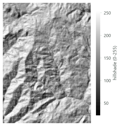
raster.terrain computes measures of a surface with GDAL's gdaldem: slope (degrees by default; percent with
options = "-p"), aspect, hillshade, TRI (terrain ruggedness), TPI (topographic position) and
roughness. Slope and the other gradients use the 3 x 3 cells around each cell (Horn's method; Horn, 1981), so
the surface must be in metres (see Coordinate systems):
Model file (TOML)
format = "terraflux/1"

[[nodes]]
id = "elevation"
op = "raster.read"
params = { path = "orelevation.tif" }

[[nodes]]
id = "elevation_utm"
op = "raster.reproject"
inputs = { raster = "elevation.raster" }
params = { crs = "EPSG:32610", resolution = 30, path = "elevation_utm.tif" }

[[nodes]]
id = "slope"
op = "raster.terrain"
inputs = { raster = "elevation_utm.raster" }
params = { measure = "slope", path = "slope.tif" }
note = "Degrees, by Horn's method."

[[nodes]]
id = "hillshade"
op = "raster.terrain"
inputs = { raster = "elevation_utm.raster" }
params = { measure = "hillshade", path = "hillshade.tif" }
note = "The relief lit from the north-west, 0 to 255: for maps, not for analysis."

Save the results#
raster.write: a GeoTIFF, in the smallest type#
raster.write writes a map, a stack (a band per map), the maps of a loop (a band per step) or rasters on disk
(copied block by block, whatever their size) to a GeoTIFF. Its settings are path (relative to the model's
folder) and type, the cell type: u8, i8, u16, i16, u32, i32, u64, i64, f32 or f64. Without
type it chooses the smallest type that holds the values: u8 for classes up to 255, f32 or f64 for
decimals. The files are compressed (Deflate). Here are the six groups of CORINE (2000 x 2000 cells) written in
three types:
| Type | Uncompressed | File written |
|---|---|---|
u8 (chosen by default) |
4.0 MB | 115 KB |
i32 |
16.0 MB | 171 KB |
f64 |
32.0 MB | 221 KB |
Compression hides most of the difference on disk for a map of few classes, but not in memory, where a map takes
its uncompressed size. Use whole-number types for classes and f32 for decimal values; f64 is rarely needed.
A map written from a raster.legend carries its names and colours into the file (as the metadata item
terraflux_legend), so Terraflux shows them when the file is read again. The bands of a stack are written with
its layers' names as their descriptions (GDAL's band names, which QGIS and R show), so the file reads back with the
same layers; a band that had no name in the file it came from is written without one.
raster.convert: other formats, cloud-optimised GeoTIFFs#
raster.convert copies rasters into another format or type with GDAL's gdal_translate: format is GDAL's name
(GTiff, COG, HFA for Erdas .img, netCDF, KEA...), type GDAL's type names (Byte, Int16, UInt16,
Int32, Float32, Float64...) and options more of gdal_translate's options. A COG (cloud-optimised
GeoTIFF) is a GeoTIFF arranged in tiles with smaller copies of itself (overviews), so that a viewer or a web
service can read just the part and the zoom it needs:
Model file (TOML)
format = "terraflux/1"

[[nodes]]
id = "groups"
op = "raster.read"
params = { path = "groups.tif" }

[[nodes]]
id = "cog"
op = "raster.convert"
inputs = { raster = "groups.raster" }
params = { format = "COG", path = "groups_cog.tif" }
note = "Tiles of 512 x 512 cells, overviews at 1/2 and 1/4."
The COG of the six groups is 202 KB, with tiles of 512 x 512 cells and overviews at ½ and ¼ of the resolution: larger than the plain GeoTIFF, much faster to show over a network. Publish maps as COGs; keep plain GeoTIFFs for work.
Saving from the viewer#
You do not need a write node to keep a map you are looking at. In the viewer's header, Save output offers
As a file... (a GeoTIFF for maps, a GeoPackage for vectors, CSV or JSON for tables and values, written in the
background) and, for maps, As a file, and a write node in the model..., which also adds a raster.write node
so that the model writes it again at every run. Save as a raster... in the Operators pane adds such a node after
the node selected.
Opening the results in QGIS#
File > Export to QGIS... (or Save output > In a QGIS project... in the viewer) lists the maps and vector
layers of the run; tick those you want (the model's outputs, the map shown and the vector layers drawn over it are
ticked at first) and choose a folder. Terraflux writes each map as a GeoTIFF and each vector layer as a GeoPackage,
with a QGIS project that opens them all (.qgz, as QGIS saves its own, or .qgs, the same project as text: a
choice in the window), in the colours you see in Terraflux: the classes as a paletted map with their names (those of
the legend you gave, or MSPA's), values on the same ramp from the same minimum to the same maximum, and the vector
layers as the viewer draws them over the map (their colour, fill and line width; by an attribute, a colour per class
or ranges of its numbers along the ramp). A vector layer ticked has its own options under it: labels by one of
its attributes, its points' marker (a circle, square, triangle, diamond, star, cross, pentagon or hexagon) and
as rules, its style written as QGIS's rules (a rule each class or range, and one for the features of none) to
change in QGIS rule by rule. Open in QGIS
opens the project. A raster read from a file is referred to where it is, not copied, and each GeoTIFF written has
its style beside it (a .qml of the same name), which QGIS uses when you add the file to another project by hand.
Common pitfalls#
- Ranges that overlap or leave gaps.
0..10 -> 1and10..20 -> 2both take 10 (the first rule wins);0..9 -> 1and10..20 -> 2leave 9.5 unchanged on a decimal map. A rule*catches what is left. - Forgetting no data. No rule touches cells without data, not even
*. If they should become a value, useraster.calcwithcoalesce(x, 0)(or0 if isnull(x) else x). - Radii in cells, not metres. Convert the distance you mean by the cell size.
- Integer division and types. A share computed from whole numbers is fine in
raster.calc(it computes in decimals), but writing it withtype = "u8"rounds it to 0 or 1. Letraster.writechoose, or sayf32. - Hillshades in analyses. A hillshade depends on an arbitrary light direction; use slope, aspect or topographic position as variables.
Going further#
- The raster calculator: the language of raster.calc, with a playground.
- Your first model: nodes, ports, the cache and the model file.
- Map algebra in the Building models tutorials, and Surface metrics.
- The operators:
raster.reclassify,raster.calc,raster.fill,raster.terrain,raster.write,raster.convert,raster.legend.
References#
- Horn, B. K. P. (1981). Hill shading and the reflectance map. Proceedings of the IEEE, 69(1), 14–47. https://doi.org/10.1109/PROC.1981.11918
- Tomlin, C. D. (1990). Geographic Information Systems and Cartographic Modeling. Prentice Hall.