Wetness, stream power and sediment connectivity

In this part you compute the terrain indices that ecologists use most as proxies of soil water and erosion: the topographic wetness index, the stream power index and the sediment transport index, all three built from the contributing area of part 1 and the local slope. Then you map the index of connectivity, which asks how easily sediment from each hillslope reaches a stream, give it a cover weight from a vegetation map, and see what clearing the riparian forest would do to it. At the end you will know what each index measures, which flow method to use for each, and how to report them so that others can reproduce your numbers.

The idea#

Two numbers describe the water arriving at a point of a hillslope: how much land drains to it, and how steep it is there. Much land and a gentle slope: water collects faster than it drains away, and the soil stays wet. Much land and a steep slope: the water runs fast and has power to erode. Little land: the soil drains and dries. The indices of this page are combinations of these two numbers.

The land is measured by the specific contributing area \( a \): the area that drains through a cell, divided by the width of the contour it crosses (the width of a cell), in m²/m (part 1, units = sca). Dividing by the width makes it independent of the resolution: it is the area that drains through each metre of contour. The slope \( \beta \) is the local slope of the cell, from Horn's (1981) method.

Moore, Grayson & Ladson (1991) reviewed the family of such compound terrain indices and their uses in hydrology, geomorphology and biology. Two others, for erosion:

The last index is about connections rather than amounts. Borselli, Cassi & Torri (2008) asked how likely sediment eroded on a cell is to reach a stream, and answered with the index of connectivity (IC); Cavalli et al. (2013) adapted it to high-resolution DEMs of Alpine catchments, and InVEST's sediment delivery ratio model uses it to decide what share of each cell's soil loss reaches the streams (Hamel et al., 2015).

When to use it#

• Soil moisture and wetland plants. TWI is one of the most common covariates of species distribution models of plants, bryophytes and amphibians, and of maps of wet soils and peat. In temperate forest plots, Kopecký, Macek & Wild (2021) found that a TWI computed with FD8 explained more than twice the variation in measured soil moisture and in the composition of vascular plants and bryophytes than one computed with D8.
• Where gullies and erosion start. High SPI marks the hollows and channel heads where concentrated flow can erode; STI is a map of the LS factor for soil loss studies.
• Where to put buffers and restoration. IC shows the hillslopes whose sediment reaches the streams most easily: the first candidates for riparian buffers, reforestation or erosion control, and the places where a clearing would hurt the streams most.
• InVEST. hydro.connectivity_index is the IC of InVEST's sediment delivery ratio model, computed the same way; use it to understand that model or to build variants of it (Ecosystem services).

What they are not: TWI assumes a water table parallel to the surface and soils of uniform conductivity, so it works best in humid landscapes with shallow soils over impermeable rock and worst on deep, permeable or flat land. SPI and STI rank places by erosion potential; they are not soil loss in tonnes (for that, see the RUSLE of InVEST's services.sdr or SWAT+ in part 4). IC is a relative index: compare it within a map and between scenarios on the same map, not as an absolute measure between regions.

What you need#

• The filled DEM of part 1: filled.tif, the Oregon SRTM elevation reprojected to UTM 10N in cells of 30 m and filled, as part 1's save_filled node writes it.
• A projected DEM, for the index of connectivity: it takes the size of its cells from the map's coordinates as they are, so a map in degrees would give areas in square degrees. TWI, SPI and STI take cells in metres either way.
• A cover weight for IC: here made from the summer NDVI of the same area (ndvi.tif, as in part 1), forest above 0.55, open land below.

Build the model#

Wetness, stream power and sediment transport#

format = "terraflux/1"

[[nodes]]
id = "filled"
op = "raster.read"
params = { path = "filled.tif" }

[[nodes]]
id = "twi"
op = "hydro.twi"
inputs = { dem = "filled.raster" }
params = { method = "fd8" }
note = "ln(a / tan slope)"

[[nodes]]
id = "spi"
op = "hydro.spi"
inputs = { dem = "filled.raster" }
note = "a x tan slope"

[[nodes]]
id = "sti"
op = "hydro.sti"
inputs = { dem = "filled.raster" }
params = { sca_exponent = 0.4, slope_exponent = 1.3 }
note = "The LS factor from the area."

Each of the three operators computes its two parts itself from the DEM: the specific contributing area by the accumulation method (fd8 by default, also quinn, dinf, d8 and mfd, as in part 1) and the slope by Horn's method. The results are WhiteboxTools' WetnessIndex, StreamPowerIndex and SedimentTransportIndex cell for cell. The other settings:

• min_slope (hydro.twi only): a floor for \( \tan \beta \). On perfectly flat cells \( \tan \beta = 0 \) and the TWI is infinite, so they get no value (here 155 cells, the flat floors of filled depressions). A floor such as 0.001 gives them a high, finite value.
• sca_exponent and slope_exponent (hydro.sti only): \( m \) and \( n \). Moore & Burch's 0.4 and 1.3 are the usual values.
• flats: drain flat areas (on by default; leave it on with a filled DEM).

Two optional inputs replace the parts: sca, a specific contributing area made your own way, and slope, a slope in degrees. That is how to follow a recipe exactly. Kopecký et al. (2021) recommend FD8 with a flow dispersion (the exponent of hydro.flow_accumulation) close to 1.0, the flow width equal to the cell size, and the local slope; Terraflux's default exponent is Freeman's 1.1. For their recipe:

format = "terraflux/1"

[[nodes]]
id = "filled"
op = "raster.read"
params = { path = "filled.tif" }

[[nodes]]
id = "sca"
op = "hydro.flow_accumulation"
inputs = { dem = "filled.raster" }
params = { method = "fd8", exponent = 1.0, units = "sca" }
note = "m²/m, the area per metre of contour."

[[nodes]]
id = "twi"
op = "hydro.twi"
inputs = { dem = "filled.raster", sca = "sca.map" }

On this map the difference is small (the two TWIs correlate at 0.9999, the recipe's is higher by 0.02 on average), but stating it makes your index reproducible.

The index of connectivity#

format = "terraflux/1"

[[nodes]]
id = "filled"
op = "raster.read"
params = { path = "filled.tif" }

[[nodes]]
id = "ndvi_read"
op = "raster.read"
params = { path = "ndvi.tif" }

[[nodes]]
id = "ndvi"
op = "raster.reproject"
inputs = { raster = "ndvi_read.raster" }
params = { crs = "EPSG:32610", resolution = 30, extent = [500010, 4760850, 508110, 4771920], resampling = "bilinear" }

[[nodes]]
id = "cover"
op = "raster.calc"
inputs = { n = "ndvi.raster" }
params = { expression = "0.003 if n > 0.55 else 0.05" }
note = "W: a USLE C per cover (illustrative)."

[[nodes]]
id = "ic"
op = "hydro.connectivity_index"
inputs = { dem = "filled.raster", weight = "cover.map" }
params = { threshold = 500, method = "mfd" }
note = "log10(D_up / D_dn), as InVEST's SDR."

The two weights are illustrative values of the order of a closed forest's and a grassland's C; in a real study, take them from the biophysical table of your land uses (the same table InVEST's sediment model reads) and say where they come from.

hydro.connectivity_index reproduces what InVEST's sediment delivery ratio model does inside: it fills the DEM, routes water by InVEST's multiple flow directions (method mfd, the default, or d8), computes the slope gradient as InVEST does and bounds it between 0.005 and 1, raises weights below 0.001 to 0.001, and finds the streams either from the streams input (1 on the streams) or as the cells whose accumulation reaches the threshold, in cells. The streams have no value: IC is about the way to them.

A scenario: the riparian forest cleared#

What if the forest along the streams were cleared? Use the HAND of part 2 to find the valley floors and give them the weight of open land:

format = "terraflux/1"

[[nodes]]
id = "filled"
op = "raster.read"
params = { path = "filled.tif" }

[[nodes]]
id = "ndvi_read"
op = "raster.read"
params = { path = "ndvi.tif" }

[[nodes]]
id = "ndvi"
op = "raster.reproject"
inputs = { raster = "ndvi_read.raster" }
params = { crs = "EPSG:32610", resolution = 30, extent = [500010, 4760850, 508110, 4771920], resampling = "bilinear" }

[[nodes]]
id = "cover"
op = "raster.calc"
inputs = { n = "ndvi.raster" }
params = { expression = "0.003 if n > 0.55 else 0.05" }

[[nodes]]
id = "hand"
op = "hydro.hand"
inputs = { dem = "filled.raster" }
params = { threshold = 500 }

[[nodes]]
id = "cleared"
op = "raster.calc"
inputs = { c = "cover.map", h = "hand.map" }
params = { expression = "0.05 if h < 20 else c" }

[[nodes]]
id = "ic"
op = "hydro.connectivity_index"
inputs = { dem = "filled.raster", weight = "cover.map" }
params = { threshold = 500 }

[[nodes]]
id = "ic_cleared"
op = "hydro.connectivity_index"
inputs = { dem = "filled.raster", weight = "cleared.map" }
params = { threshold = 500 }

terraflux check indices.toml
terraflux run indices.toml --out output

Read the results#

Wetness. The TWI (FD8) of this map goes from about 5 on the ridges to 13 in the main valleys (1^st and 99^th percentiles); its median is 6.4. The streams draw continuous dark lines, and the hollows at their heads fan out in lighter blue: the zones of the hillslopes where water converges. Valley floors are much wetter than the rest: the cells less than 5 m above their stream (part 2) have a mean TWI of 11.2, the others 6.7, and the mean falls steadily as HAND rises.

TWI and HAND are related but not interchangeable: their correlation across the map is −0.42. HAND says how high a cell is above the drainage; TWI how much water converges on it. A hollow high on a slope can have a high TWI and a large HAND.

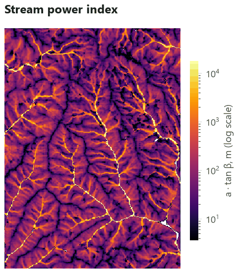
Stream power and sediment transport. SPI spans five orders of magnitude (median 69, the main river several hundred thousand), so map and analyse its logarithm. Its highest values are on the streams themselves, where the index has little meaning for hillslope erosion: mask the streams, or read SPI on the hillslopes and channel heads. STI has a median of 17.8 and 90 % of the map below 39: this steep terrain is, by its shape alone, an erosive one; the cover (forest) is what protects it.

Connectivity. IC ranges from about −7.1 to −3.6 here (1^st to 99^th percentiles); only the differences mean something. Red cells (high IC) are hillslopes close to a stream along steep paths, and the open patches, whose larger weight (a less protective cover) raises the upslope component and shortens the downslope one; blue cells (low IC) are ridges far from any stream, behind long forested slopes.

Enlarge

Clearing the riparian forest turns 11 % more of the map into open land, all of it on the valley floors. Drag the handle:

Today

Riparian forest cleared

On the valley floors (HAND under 20 m) the mean IC rises from −4.71 to −3.19, 1.5 units: sediment reaches the streams some 30 times more easily (\( 10^{1.5} \)). On the slopes above, untouched, it still rises by 0.34 (a factor of 2), because their path to the streams now crosses cleared land. That is the case for riparian buffers in one figure: a strip of forest along the streams protects them from the sediment of the whole hillslope above.

Settings that change the answer#

The flow method matters for TWI more than any other setting. Move the slider:

Enlarge

PlayAccumulation method

The TWI by D8 correlates with the TWI by FD8 at only 0.83 across the map. In a species distribution model, that is a different covariate. Prefer FD8 (Kopecký et al., 2021) unless you have a reason, such as consistency with an earlier study, and test the choice against field measurements when you have them; Sørensen, Zinko & Seibert (2006) found that the best method varied with the variable (species richness, soil pH, groundwater, soil moisture) and the site.

The resolution changes everything: \( a \) grows and slopes flatten as cells grow, and a TWI from a 30 m DEM cannot see the microtopography that a lidar DEM of 1 m sees. Compare TWI only between maps of the same resolution and method.

The stream threshold of IC moves where the paths end. With streams from 9 ha, the paths are shorter and the mean IC is −5.12; from 45 ha, −5.48; from 225 ha, −5.88. The pattern changes little; the values shift. The routing matters less: IC by D8 routing correlates with IC by mfd at 0.86. And the weights decide the contrast between land uses: they are the part to justify best.

Common pitfalls#

• An unprojected DEM for IC. hydro.connectivity_index takes the cell size from the map's coordinates; in degrees, the areas and distances are wrong. Reproject first.
• Flat cells. Without min_slope, filled flats have no TWI. A model fitted on the cells with a value silently leaves out the wettest places (filled valley bottoms). Set a small floor, or fill the holes.
• SPI on its natural scale. It is so skewed that a regression on it is driven by a few stream cells. Take its logarithm (with a small constant if some cells are 0).
• Comparing with other software. SAGA's "SAGA wetness index", ArcGIS recipes and WhiteboxTools' tools give different numbers for the "same" TWI: different accumulation methods, flow widths and slopes. Report your method, and compare like with like.
• IC between regions. IC depends on the units, the resolution and the weights. Compare scenarios on one map, not absolute values between studies.
• Weights in the wrong range. \( W \) is a cover factor between 0 and 1 (InVEST raises values below 0.001 to 0.001). A weight of 1 for forest and 10 for crops is not a C factor.

Going further#

• Part 1: Depressions, flow directions and flow accumulation and part 2: Streams, watersheds and HAND.
• Part 4: Watershed simulation with SWAT+: erosion and water in tonnes and millimetres, day by day.
• Terrain from an elevation model: slope, curvature and topographic position, the other terrain covariates.
• Species distributions: TWI and HAND as covariates.
• Ecosystem services: InVEST's sediment delivery ratio model, which uses this IC.
• The operators' reference: hydro.twi, hydro.spi, hydro.sti, hydro.connectivity_index, services.sdr.

References#

• Beven, K. J., & Kirkby, M. J. (1979). A physically based, variable contributing area model of basin hydrology. Hydrological Sciences Bulletin, 24(1), 43–69. https://doi.org/10.1080/02626667909491834
• Borselli, L., Cassi, P., & Torri, D. (2008). Prolegomena to sediment and flow connectivity in the landscape: A GIS and field numerical assessment. Catena, 75(3), 268–277. https://doi.org/10.1016/j.catena.2008.07.006
• Cavalli, M., Trevisani, S., Comiti, F., & Marchi, L. (2013). Geomorphometric assessment of spatial sediment connectivity in small Alpine catchments. Geomorphology, 188, 31–41. https://doi.org/10.1016/j.geomorph.2012.05.007
• Hamel, P., Chaplin-Kramer, R., Sim, S., & Mueller, C. (2015). A new approach to modeling the sediment retention service (InVEST 3.0): Case study of the Cape Fear catchment, North Carolina, USA. Science of the Total Environment, 524–525, 166–177. https://doi.org/10.1016/j.scitotenv.2015.04.027
• Horn, B. K. P. (1981). Hill shading and the reflectance map. Proceedings of the IEEE, 69(1), 14–47. https://doi.org/10.1109/PROC.1981.11918
• Kopecký, M., Macek, M., & Wild, J. (2021). Topographic Wetness Index calculation guidelines based on measured soil moisture and plant species composition. Science of the Total Environment, 757, 143785. https://doi.org/10.1016/j.scitotenv.2020.143785
• Moore, I. D., & Burch, G. J. (1986). Physical basis of the length-slope factor in the Universal Soil Loss Equation. Soil Science Society of America Journal, 50(5), 1294–1298. https://doi.org/10.2136/sssaj1986.03615995005000050042x
• Moore, I. D., Grayson, R. B., & Ladson, A. R. (1991). Digital terrain modelling: A review of hydrological, geomorphological, and biological applications. Hydrological Processes, 5(1), 3–30. https://doi.org/10.1002/hyp.3360050103
• Sørensen, R., Zinko, U., & Seibert, J. (2006). On the calculation of the topographic wetness index: Evaluation of different methods based on field observations. Hydrology and Earth System Sciences, 10(1), 101–112. https://doi.org/10.5194/hess-10-101-2006