

Continuous surfaces, part 3 of 4
Landforms with geomorphons
Classify every cell of an elevation model into one of ten landforms (peak, ridge, spur, slope, hollow, valley, pit...) by looking along eight lines of sight, and learn how the search radius sets the scale of the landforms you map.
- Level
- Intermediate
- Time
- 40 min
In this tutorial you classify the mountains of the first part of the series into landforms: every cell of the elevation model becomes a peak, a ridge, a shoulder, a spur, a slope, a hollow, a footslope, a valley, a pit or a flat. You will see how the method decides, by looking from each cell along eight lines of sight; build the model in Terraflux; read the map, the patterns and the measures it gives; and move the search radius to watch the landforms change from gullies and knolls to whole ridges and valleys. At the end you will have a categorical map of landforms ready to use as a covariate in a species distribution or land change model, and you will know which settings to report.
The idea#
The terrain indices of the first part (slope, curvature, the topographic position index) describe the ground around a cell through a window: 3 × 3 cells for slope and curvature, a square or a circle for TPI. Two things make windows awkward for classifying landforms. A small window sees only a small part of a landform (a 3 × 3 window on a 30 m elevation model sees 90 m of a ridge that may be 2 km long), and a large window averages the heights inside it, so that a narrow ridge on a broad slope disappears in the mean. To name a landform you would rather know, from where you stand, where the ground goes up and where it goes down, as a geomorphologist does in the field.
Jasiewicz & Stepinski (2013), building on a short paper of 2011 (Stepinski & Jasiewicz, 2011), proposed exactly that. From each cell they look along the eight compass directions, up to a distance \( L \), and ask in each direction whether the terrain is higher than the cell, lower, or about level. Eight answers, each one of three symbols, make a geomorphon (a "form element"), and a geomorphon names a landform: if the terrain falls in all eight directions, the cell is a peak; if it rises in all eight, a pit; if it falls in six and rises in two (on either side of a crest line), a ridge. The angles they use build on the openness of Yokoyama et al. (2002), a measure of how much of the sky or of the ground a point "sees" along lines of sight.

Key idea: one direction of a geomorphon
Along direction \( i \) (north, north-east, east...), consider every cell from the first one (or, with a skip, from a little further) up to the search distance \( L \). For each, the angle of the line of sight from the cell to it, above (positive) or below (negative) the horizontal: \( \beta = \arctan(\Delta z / d) \), with \( \Delta z \) the difference of elevation and \( d \) the horizontal distance. Keep the largest, \( \beta^{+}_i \), and the smallest, \( \beta^{-}_i \). (Jasiewicz & Stepinski express them as the zenith angle \( 90° - \beta^{+}_i \), between the vertical above the cell and its highest line of sight, and the nadir angle \( 90° + \beta^{-}_i \), between the vertical below the cell and its lowest one.)
With a flatness threshold \( t \) (1° by default), the direction is:
- level (0) if neither \( |\beta^{+}_i| \) nor \( |\beta^{-}_i| \) exceeds \( t \): the terrain looks flat;
- higher (+) if \( |\beta^{+}_i| > |\beta^{-}_i| \): the terrain rises more steeply than it falls;
- lower (−) if \( |\beta^{-}_i| > |\beta^{+}_i| \).
This is the comparison of GRASS GIS's r.geomorphon (its default, anglev1), which Terraflux reproduces.
What makes the method fast and robust is what comes next. The eight symbols of a cell are counted: how many directions are higher (\( n^{+} \)) and how many lower (\( n^{-} \)). The pair \( (n^{+}, n^{-}) \), whatever the directions they point to, names one of ten landforms through a lookup table:

Read the table from its corners. No direction lower and none higher (top left): flat. All eight lower: peak; all eight higher: pit. Six or seven lower: ridge; six or seven higher: valley. In the middle, where the terrain rises on one side and falls on the other, is the slope; a slope with more directions falling than rising bends outwards like the nose of a hill, a spur; one with more rising than falling bends inwards, a hollow. Where many directions are level and a few fall, the cell is at the edge of a flat, about to drop: a shoulder; where many are level and a few rise, it is at the foot of a rise: a footslope.
The real patterns behind those ten names are more than ten. Up to rotation and reflection (a ridge running north and one running east are the same landform) there are 498 different geomorphons. Here is the commonest one of each landform on the map of this tutorial:

The slope (four + in a row, four − in a row) is a plane tilted one way; the spur has one − more, the hollow one + more; the ridge has two + on opposite sides of six −.
Two things set geomorphons apart from window-based indices:
- The scale is the search distance \( L \), and it can be large without blurring. The method keeps only the steepest lines of sight, not a mean, so a narrow ridge is still a ridge with \( L \) = 2 km, and one map can hold landforms of very different sizes, a gully and a whole valley (Jasiewicz & Stepinski, 2013).
- It is a pattern, not a number. There is no threshold to choose on the output: the classes come from the counts, and they mean the same thing in a lowland and a mountain range (only the flatness threshold depends on the relief).
When to use it#
Use geomorphons when you want named landforms rather than continuous indices:
- As covariates of species distribution models. Many plants and animals sort themselves along slope position: ridge-top shrubs, valley-bottom riparian species, cliff nesters on spurs and peaks. A map of ten landforms (or a few indicators made from it, such as "ridge or peak") is easy to interpret in a fitted model. Amatulli et al. (2018) computed geomorphons with other topographic variables for the whole world, at 1 km and coarser, for environmental and biodiversity modelling, and Amatulli et al. (2020) at 90 m (Geomorpho90m), so that they can be used as predictors anywhere (see Species distributions).
- As drivers of land change. Deforestation and farming follow the terrain: flat valley floors and gentle slopes are cleared first, ridges and steep spurs last. A landform map is a natural categorical driver for the models of Land change simulation (as a static variable in Dinamica's weights of evidence, or a factor in a regression).
- For soils and geomorphology. Libohova et al. (2016) used geomorphons to predict landforms and soil properties on a glacial moraine in Indiana; Robaina et al. (2017) used them to classify the landforms of the state of Tocantins, Brazil.
- To stratify field work. Sampling plots by landform spreads them over ridges, slopes and valleys.
What geomorphons are not: they are not a hydrological analysis (a "valley" is a cell lower than its surroundings in six or seven directions, not a stream; for flow, see Terrain hydrology), and they are not a slope map: a gentle valley and a gorge are both valleys. Combine them with slope when steepness matters. For continuous position, the TPI and the slope positions of the first part remain useful; for the protected hilltops of Brazil's Forest Code, see the next part.
What you need#
- An elevation model in projected coordinates. Terraflux measures the lines of sight in map units, so the cells
must be in metres:
surface.geomorphonsrefuses a map in longitude and latitude ("geomorphons need a projected DEM (distances in map units): reproject it first"). Here:orelevation.tif, the SRTM elevation of south-western Oregon (about 30 m) of the first part, saved aselevation.tifand reprojected to UTM zone 10N withraster.reproject, exactly as there. For your own data use the UTM zone of the area (for most of Brazil, SIRGAS 2000 / UTM, EPSG:31978 to EPSG:31985) or an equal-area projection. - A resolution matched to your landforms. The search radius is counted in cells by default: 20 cells is 600 m on a 30 m model and 20 m on a 1 m lidar model. Free global models (SRTM, Copernicus GLO-30, ALOS AW3D30) have cells of about 30 m.
- A margin. Lines of sight stop at the edge of the map (see the pitfalls): read the model with a margin of the search radius around your study area.
Build the model#
Read, reproject and classify#
- In the library, open IO and click
raster.read; set path toelevation.tifand rename the nodedem(Ctrl+R). With it selected, addraster.reprojectfrom Data preparation, namedelevation, with crs =EPSG:32610, resolution =30, resampling =bilinearand extent =[500010, 4760850, 508110, 4771920](the reason for each is in the first part). - With
elevationselected, open the subject Surface metrics and clicksurface.geomorphons: it comes connected through itsdeminput. Rename itlandformsand set search to20. - Press Ctrl+Enter. The Viewer shows the
formsoutput: the ten landforms with their names in the legend, in the colours of GRASS GIS (the application recognises this output). Its header lists the node's other outputs (ternary,share...) to choose from.
Model file (TOML)
format = "terraflux/1"

[[nodes]]
id = "dem"
op = "raster.read"
params = { path = "elevation.tif" }
note = "SRTM elevation, 1 arc-second, longitude and latitude."

[[nodes]]
id = "elevation"
op = "raster.reproject"
inputs = { raster = "dem.raster" }
params = { crs = "EPSG:32610", resolution = 30, extent = [500010, 4760850, 508110, 4771920], resampling = "bilinear" }
note = "Square cells of 30 m: geomorphons need metres."

[[nodes]]
id = "landforms"
op = "surface.geomorphons"
inputs = { dem = "elevation.raster" }
params = { search = 20 }
note = "Eight lines of sight of 600 m from every cell."
Node 3 has five outputs you will use, and eight more with measures (below):
| Output | What it holds |
|---|---|
forms |
the landform of each cell, 1 flat, 2 peak, 3 ridge, 4 shoulder, 5 spur, 6 slope, 7 hollow, 8 footslope, 9 valley, 10 pit |
ternary |
the geomorphon itself: its eight symbols as a number in base 3, the smallest of its rotations and reflections (498 possible codes between 0 and 6560) |
positive, negative |
the directions in which the terrain is higher (or lower) than the flatness threshold, as eight bits, the smallest of their rotations (0 to 255) |
share |
a table with a row per landform: form (its code), cells, share (a fraction of the cells with a form) |
The settings of surface.geomorphons, and what they mean on the ground:
- search: the outer search radius \( L \), 3 by default, in cells (or in map units with units =
map). This is the scale of the landforms: a valley is a valley within this distance. With units =map, search =600gives exactly the same map as 20 cells of 30 m here (every cell identical; it is GRASS's-m). - skip: an inner radius not looked at, 0 by default. With skip = 3 the lines of sight start 4 cells away, so that bumps and noise within 90 m of a cell do not decide its form: GRASS's manual describes it as removing forms smaller than the skip.
- flat: the flatness threshold \( t \) in degrees, 1 by default. Lines of sight within \( t \) of the horizon count as level. Raise it on rough or noisy models to find flats; lower it on very coarse ones (GRASS's manual suggests a smaller threshold for cells larger than about 1 km).
- dist: the flatness distance, 0 (none) by default. Beyond it the threshold is no longer an angle but a height, \( \tan(t) \times \text{dist} \): far points count as higher or lower when they differ by more than that height, however small their angle. It keeps distant low hills from being "level" on large search radii. It must lie between skip and search, or it is ignored.
- comparison: how the two angles decide a direction:
anglev1(the original, the default),anglev2andanglev2_distance, which GRASS describes as better handling of the threshold and of angles up and down that are exactly equal (the second breaking such ties by the distance of the two points). On this mapanglev2changes 1.2 % of the cells: all 185 shoulders become slopes, nearly all 284 footslopes become valleys, and some slopes become valleys or hollows. Expect larger differences on models with whole-metre heights and on terraced or synthetic surfaces, where equal angles are common. - extended: GRASS's "extended form correction" (
-e). When the search radius is larger than 10 cells, a cell classified as a ridge, peak, shoulder or footslope is looked at again with half the radius (at least 4 cells): a ridge or a peak takes the form of the shorter look, and a shoulder or footslope becomes flat if the shorter look finds it flat. At 40 cells it changes 2.9 % of this map: 29 % of the peaks become ridges and 16 % of the ridges become spurs, crests that looked sharper from far away than from close by. - measures: also compute the eight measures of each geomorphon (below); off by default because they take time.
Show it over the relief, save it, and make a covariate#
- Select
elevationand addraster.terrainwith measure =hillshade, namedshade. Double-clickshadeto keep the relief as a layer of the Viewer, then clicklandformsand, in Layers, keep itsformstoo (📌) with opacity =0.75: the landforms drawn over the relief. Keep the view with Plots › Save as a new plot, titledLandforms. - Add a
table.writeafterlandforms, itstableinput from theshareoutput, path =landforms.csv. - Add a
raster.calcnamedcrests(subject Map algebra), connectlandforms'sformsto an input you namef, and write1 if f == 2 or f == 3 else 0: 1 on peaks and ridges, 0 elsewhere.
Model file (TOML)
format = "terraflux/1"

[[nodes]]
id = "dem"
op = "raster.read"
params = { path = "elevation.tif" }

[[nodes]]
id = "elevation"
op = "raster.reproject"
inputs = { raster = "dem.raster" }
params = { crs = "EPSG:32610", resolution = 30, extent = [500010, 4760850, 508110, 4771920], resampling = "bilinear" }

[[nodes]]
id = "landforms"
op = "surface.geomorphons"
inputs = { dem = "elevation.raster" }
params = { search = 20 }

[[nodes]]
id = "shade"
op = "raster.terrain"
inputs = { raster = "elevation.raster" }
params = { measure = "hillshade" }

[[nodes]]
id = "save"
op = "table.write"
inputs = { table = "landforms.share" }
params = { path = "landforms.csv" }

[[nodes]]
id = "crests"
op = "raster.calc"
inputs = { f = "landforms.forms" }
params = { expression = "1 if f == 2 or f == 3 else 0" }
note = "1 on peaks and ridges."

[[plots]]
id = "relief"
title = "Relief"
layers = [{ from = "shade.raster" }]

[[plots]]
id = "map"
title = "Landforms"
layers = [{ from = "shade.raster" }, { from = "landforms.forms", opacity = 0.75 }]
Press F5 to run the whole model. The Plot Landforms (the Viewer's Plots menu) shows the classes over
the relief; the legend names them. To keep the map as a file, use Save output in the Viewer's header or add
a raster.write node after landforms's forms.
Save the model as landforms.toml beside elevation.tif, add a raster.write node for the maps you want on
disk, and run:
terraflux check landforms.toml
terraflux run landforms.toml --out output
The indicator in node 6 is how a categorical map usually enters a regression: one 0/1 map per landform (or group
of landforms) you want a coefficient for. Most species distribution methods also accept the forms map directly as
a categorical predictor; then the coefficients are relative to a reference class (choose a common one, here the
slope).
Read the results#
The landform map#

The map reads like a sketch of the relief. Red ridges run along every crest and its side spurs, ending in dark peaks on the summits; blue valleys follow the streams from the main valley in the south-east up into each side valley, ending in black pits where a valley floor is lower than everything around it within 600 m (small closed depressions, or the elevation model's own errors). Between them, slopes (36 %) are flanks that rise on one side and fall on the other; spurs (22 %) and hollows (18 %) are flanks that bend outwards and inwards. Shoulders and footslopes are rare and flat cells absent: in these mountains almost no line of sight stays within 1° of the horizon.
| Code | Landform | Cells | Share (%) |
|---|---|---|---|
| 1 | Flat | 0 | 0 |
| 2 | Peak | 1,360 | 1.38 |
| 3 | Ridge | 10,864 | 11.05 |
| 4 | Shoulder | 185 | 0.19 |
| 5 | Spur | 21,324 | 21.68 |
| 6 | Slope | 35,567 | 36.16 |
| 7 | Hollow | 17,978 | 18.28 |
| 8 | Footslope | 284 | 0.29 |
| 9 | Valley | 9,708 | 9.87 |
| 10 | Pit | 1,086 | 1.1 |
A good sign: ridges and valleys form continuous lines, as on a topographic map, and their share is in proportion to the relief (here, about 11 % ridges and 10 % valleys). A bad sign: a speckle of peaks and pits all over the map, or ridges broken into dots, means the search radius is too small for the elevation model's noise; raise search, or use skip.
Patterns#
The ternary output keeps the geomorphon of each cell. Of the 498 possible patterns, only 63 occur on this map, and
ten account for 97 % of the cells:
| Ternary code | The eight directions (one rotation) | Higher | Lower | Landform | Share (%) |
|---|---|---|---|---|---|
| 80 | + + + + − − − − | 4 | 4 | Slope | 34.94 |
| 26 | + + + − − − − − | 3 | 5 | Spur | 21.04 |
| 242 | + + + + + − − − | 5 | 3 | Hollow | 17.79 |
| 8 | + + − − − − − − | 2 | 6 | Ridge | 7.55 |
| 728 | + + + + + + − − | 6 | 2 | Valley | 6.72 |
| 2 | + − − − − − − − | 1 | 7 | Ridge | 3.01 |
| 2,186 | + + + + + + + − | 7 | 1 | Valley | 2.74 |
| 0 | − − − − − − − − | 0 | 8 | Peak | 1.38 |
| 6,560 | + + + + + + + + | 8 | 0 | Pit | 1.1 |
| 62 | + + − + − − − − | 3 | 5 | Spur | 0.37 |
Code 80 (four directions up, then four down) is a plane, the commonest form of a mountain flank; code 0 (all eight
down) is a peak and code 6560 (all eight up) a pit. Patterns add detail to the forms: two ridges with the same counts
can differ in where their higher directions are, side by side (a ridge ending in a spur) or opposite (a crest
between two valleys). Use the ternary map when ten classes are too coarse, for instance to tell one-sided from
two-sided ridges, or as a texture of the terrain. The positive and negative maps keep only the directions that
rise (or fall), each as eight bits up to rotation: 0 for none, 255 for all.
The measures#
With measures = true, surface.geomorphons also describes each geomorphon by the points that decide its
directions (the farthest point of steepest ascent in a higher direction, of steepest descent in a lower one):
intensity: the mean height of the cell above those points, in metres: positive on peaks and ridges (here +83 m on average on peaks, +54 m on ridges), near 0 on slopes, negative in valleys (−51 m) and pits (−78 m);exposition: minus the height difference to the most different of those points, in metres;rangeandvariance: the range and the variance of their heights;- the shape of the octagon those points draw around the cell (a level direction counts at the search radius):
elongation(the ratio of its long and short sides),azimuth(the direction of its long axis, in degrees),extend(its area, as a share of the full octagon of the search radius) andwidth(its short side, in metres).
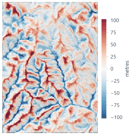
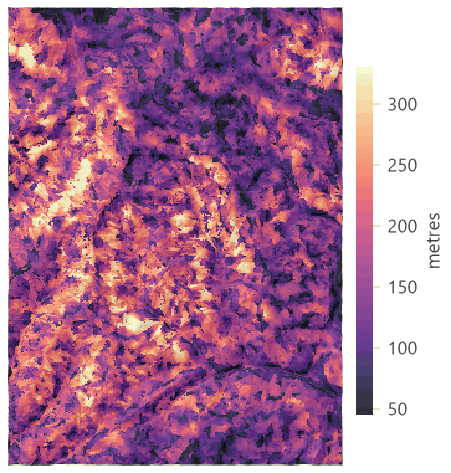


GRASS's manual marks the measures as experimental. Intensity is the easiest to read: a continuous companion of the forms, close in meaning to the TPI but measured over the lines of sight instead of a window.
How Terraflux compares with GRASS#
surface.geomorphons runs landschaft's port of r.geomorphon from GRASS GIS 8.4. On the six reference elevation
models kept with landschaft's tests (real SRTM heights, heights rounded to whole metres, holes in the data, cells of
20 × 30 m, search in map units, the extended correction, all three comparisons), its forms and patterns are those of
GRASS in all 73,500 cells where both give a value. It corrects four errors of r.geomorphon 8.4: the lines of sight
of the cells in GRASS's bottom rows stop one row short of the map's last row; GRASS's positive and negative
patterns add the numbers of the directions instead of setting their bits; its extended correction keeps the skip in
its second, shorter look although it means to drop it; and the shape of a geomorphon whose first direction (north-east)
has no point comes out as zeros. Outside these cases the values are GRASS's.
How to report#
Give the elevation model (source, resolution, projection), the method (geomorphons, Jasiewicz & Stepinski, 2013,
as implemented in GRASS GIS's r.geomorphon, here through Terraflux), the search radius in cells and in metres,
the skip, the flatness threshold and distance, the comparison, and whether the extended correction was used. Show
the map over a hillshade with the ten names in the legend, and give the share of each landform.
Settings that change the answer#
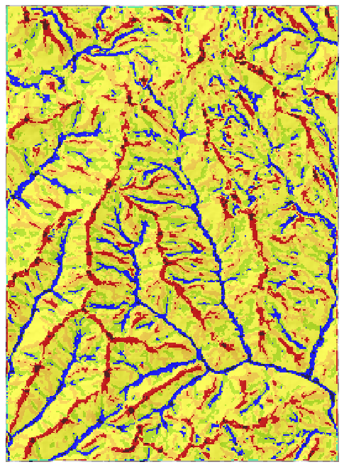
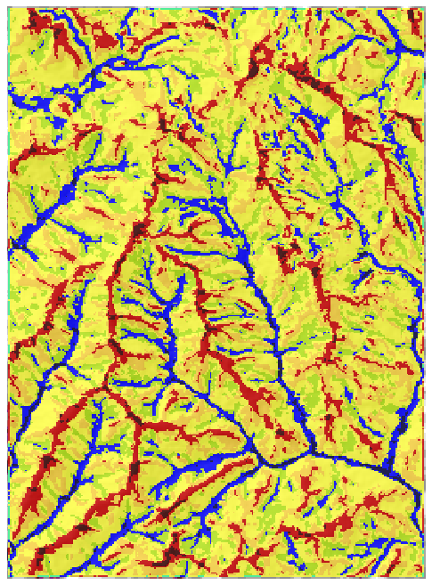
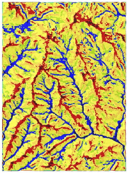
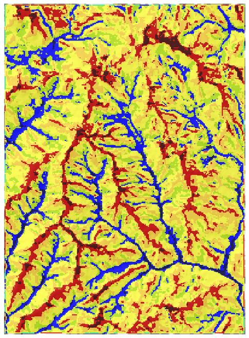
The search radius is the setting that matters. Move the slider from 3 cells (90 m) to 80 cells (2.4 km):


What to notice:
- Small radii see small landforms. At the default of 3 cells, a ridge must be a ridge within 90 m: only the sharpest crests qualify, and every small gully is a valley. Half the map is "slope".
- The map settles. From about 600 m on, the shares change by a point or two: the landforms of these mountains are a few hundred metres across, and longer lines of sight add few new ones. Look for that plateau on your own data: it marks the scale of the main landforms. GRASS's manual puts it this way: a radius \( L \) identifies correctly the landforms smaller than \( L \), and a large \( L \) identifies landforms of many sizes at once.
- Unlike a window, a larger radius costs no cells. Every frame has forms on 98.7 % of the map: lines of sight simply stop at the edge. The price is hidden: near the edges, forms are decided by shorter lines than elsewhere.
The flatness threshold matters on gentle relief. In these steep mountains no cell becomes flat even at 6°, but the slopes grow at the expense of ridges and valleys, and a few shoulders and footslopes appear where gentle crests and valley floors meet steeper flanks:
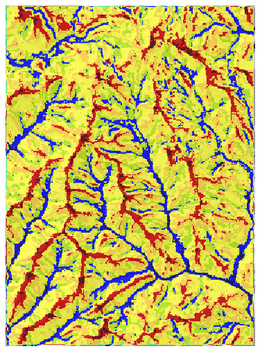
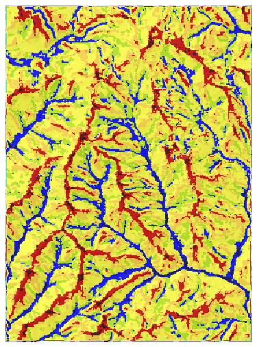
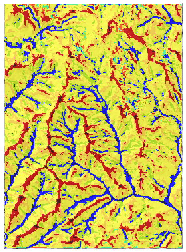
On a floodplain, a coastal plain or a plateau the threshold decides how much of the map is flat; there, try 1° to 3° and check the flats against what you know of the ground.
skip changes more than one would think: with skip = 3 at 20 cells, 37 % of the cells change form, and ridges (16.4 %) and valleys (15.5 %) widen at the expense of slopes (26.3 %): the form of a cell is now decided by the terrain from 120 m away, not by its nearest neighbours. Use it to remove noise or features smaller than the skip, and report it.
Common pitfalls#
- Longitude and latitude. The operator refuses them; reproject first, with
bilinearresampling (notnear, which makes terraces whose edges become false shoulders and footslopes). - The default radius. 3 cells is a very local look (90 m on a 30 m model). Choose the radius in metres from the landforms that matter to your question, and convert it to cells for your resolution.
- Comparing maps of different resolutions. 20 cells at 30 m (600 m) and 20 cells at 90 m (1.8 km) are different
scales; use units =
mapto keep the same distance. - Surface models. Radar elevation models (SRTM in places, other "DSMs") include the canopy and buildings: a forest edge becomes a step, a clearing a pit. Use a terrain model (bare ground) where one exists, for instance ANADEM for South America (Laipelt et al., 2024).
- Edges. Lines of sight stop at the map's edge, so cells near it are classified from fewer and shorter lines. Read a margin of the search radius around your study area and cut the map afterwards.
- Pits. Small pits in valleys are often errors of the elevation model, not real depressions. Do not interpret them without checking.
- Treating codes as numbers. The forms are classes: a mean landform of 5.9 means nothing. Use shares, indicators, or the map as a categorical variable.
Going further#
- Terrain from an elevation model: slope, aspect, TPI and Weiss's slope positions, the window-based counterpart of geomorphons.
- Hilltops protected by Brazil's Forest Code: summits, saddles and the hilltop APP, the next part.
- Species distributions and Land change simulation: use the landforms as covariates.
- The operators' reference:
surface.geomorphons,raster.reproject,raster.terrain,raster.calc.
References#
- Amatulli, G., Domisch, S., Tuanmu, M.-N., Parmentier, B., Ranipeta, A., Malczyk, J., & Jetz, W. (2018). A suite of global, cross-scale topographic variables for environmental and biodiversity modeling. Scientific Data, 5, 180040. https://doi.org/10.1038/sdata.2018.40
- Amatulli, G., McInerney, D., Sethi, T., Strobl, P., & Domisch, S. (2020). Geomorpho90m, empirical evaluation and accuracy assessment of global high-resolution geomorphometric layers. Scientific Data, 7, 162. https://doi.org/10.1038/s41597-020-0479-6
- Jasiewicz, J., & Stepinski, T. F. (2013). Geomorphons — a pattern recognition approach to classification and mapping of landforms. Geomorphology, 182, 147–156. https://doi.org/10.1016/j.geomorph.2012.11.005
- Laipelt, L., Comini de Andrade, B., Collischonn, W., de Amorim Teixeira, A., Paiva, R. C. D., & Ruhoff, A. (2024). ANADEM: A digital terrain model for South America. Remote Sensing, 16(13), 2321. https://doi.org/10.3390/rs16132321
- Libohova, Z., Winzeler, H. E., Lee, B., Schoeneberger, P. J., Datta, J., & Owens, P. R. (2016). Geomorphons: Landform and property predictions in a glacial moraine in Indiana landscapes. Catena, 142, 66–76. https://doi.org/10.1016/j.catena.2016.01.002
- Robaina, L. E. de S., Trentin, R., Cristo, S. S. V. de, & Sccoti, A. A. V. (2017). Application of the concept of geomorphons to the landform classification in Tocantins State, Brazil. Raega – O Espaço Geográfico em Análise, 41, 37. https://doi.org/10.5380/raega.v41i0.48724
- Stepinski, T. F., & Jasiewicz, J. (2011). Geomorphons — a new approach to classification of landforms. In Proceedings of Geomorphometry 2011 (pp. 109–112). Redlands, CA.
- Yokoyama, R., Shirasawa, M., & Pike, R. J. (2002). Visualizing topography by openness: A new application of image processing to digital elevation models. Photogrammetric Engineering and Remote Sensing, 68(3), 257–265.