

Habitat patterns with GuidosToolbox, part 4 of 4
From patterns to networks and change
MSPA's cores and bridges read as a network (its components, the equivalent connected area, the importance of every link and stepping stone), the change of a forest between two dates told apart from the noise at its edges, and MSPA of maps larger than memory.
- Level
- Advanced
- Time
- 60 min
- Template
- Forest gain and loss
The first three parts described one forest at one date. This last part takes MSPA three steps further. First, the cores and bridges of an MSPA map already form a network, and GuidosToolbox reads it as one: which cores are joined, how much habitat a species could reach, and which corridors and stepping stones hold the network together. Second, landscapes change, and comparing two maps cell by cell exaggerates the change at every edge; GuidosToolbox's morphological change detection tells the change of the forest's structure apart from the noise. Third, real maps are often too large for one MSPA in memory, and a tiled MSPA runs it piece by piece. All three on the forest map of part 2, with an edge 2 cells wide. At the end you will be able to rank the links of a forest network for protection and report how a forest's structure changed between two dates.
The idea#
The network inside an MSPA map#
MSPA's classes are not only a description of shapes. A core is habitat far from the edge, where a forest species can live; a bridge is a strip of habitat that joins two cores, along which it can move. Read that way, an MSPA map is a graph: the cores are its nodes and the bridges its links. Vogt et al. (2009) used MSPA's bridges to map functional connectivity, and Saura et al. (2011b) showed that combining MSPA's structural connectors with the graph indices of Conefor finds the forest corridors that matter most, in a forest of central Spain. GuidosToolbox's network analysis (GTN) does it directly on the map (Vogt & Riitters, 2017).
Cores joined by bridges, directly or through other cores, form a component: a group of habitat that a species following the bridges can travel across without leaving the forest. A component with at least one bridge is a network; a core with no bridge is an isolated core.
Key idea: the equivalent connected area and the coherence
Let \(a_1, \ldots, a_n\) be the core areas of the \(n\) components (each the sum of the cores it joins). The equivalent connected area is
the area of a single block of habitat that would offer as much reachable habitat as the whole map (Saura et al., 2011a). If every core were joined into one component, ECA would be the total core area, \(\text{ECA}_\text{max} = \sum_i a_i\). The coherence \(\text{ECA} / \text{ECA}_\text{max}\), in %, says how much of the possible connectivity the network has: 100% when all the core is one network, low when it is split into many small pieces.
\(a_i^2\) is the numerator of the probability of connectivity (PC) of Saura & Pascual-Hortal (2007) when every pair of cores in a component is reachable and every pair in different components is not. The importance of a link or a node is then the drop of that numerator, in %, when it is removed (dPC; Saura & Rubio, 2010): a bridge whose removal splits a large network has a large dPC; one that runs parallel to another (a loop of the network) has almost none.
Change, and the noise at the edges#
Two maps of the same forest at two dates never line up perfectly. A shift of a fraction of a cell between them, a different sensor or a different classifier moves every edge a little, and a cell-by-cell comparison turns every edge of the map into a strip of gain on one side and loss on the other. On a forest with as many edges as this one, that "change" can be larger than the real one. Morphological change detection (MCD) keeps as real only the change that reaches the interior of a forest or of a field: a change is structural when it is connected to cells that were deep inside the forest at the first date and deep inside the background at the second (or the reverse). The rest, thin strips of change along the edges, is labelled spurious (Vogt & Riitters, 2017).
Key idea: the elasticity of a landscape
MCD also reports the elasticity: the % change of the forest's interior (the forest more than one cell from its edge) over the % change of the whole forest,
with \(F\) the forest and \(I\) its interior at dates A and B. \(E = 1\) when the interior changes in proportion to the forest; \(E > 1\) when a loss falls on the interior more than on the edges, for example when clearings pierce large blocks; \(E < 1\) when it is mostly the edges that retreat.
Maps larger than memory#
MSPA works on the whole map at once: a cell's class can depend on cells far away (a bridge is a bridge because of the two cores at its ends). A tiled MSPA cuts the map into overlapping tiles, runs MSPA on each, and keeps the half of each overlap nearest to each tile. Near the seams the result is exact only if no object is larger than the overlap; GuidosToolbox warns that the tiled result is an approximation, and so does Terraflux.
When to use it#
- The network when the question is which corridors and stepping stones to protect or restore first, how connected the forest of a region is (ECA, coherence), or how that connectivity changed. It is structural connectivity: it follows the forest's own bridges, so it suits species that move inside the forest and rarely cross open land. For species that cross the matrix, with a dispersal distance and a resistance, use the habitat networks (Conefor's indices on distances between patches) or the circuit connectivity tutorials.
- Simple change to count gain and loss of the forest between two maps made the same way (the same sensor, the same classifier, well registered).
- Morphological change when the two maps come from different sources, or when the change of the forest's structure matters more than the area: clearings in the interior, fragmentation. Saura et al. (2011a) followed the connectivity of European forests between 1990 and 2000 in this spirit, and the US Forest Service has tracked the change of forest fragmentation over decades with GuidosToolbox's tools (Wickham et al., 2008; Riitters & Wickham, 2012).
- The change of fragmentation (FAD at two dates,
change.fad) is the subject of the fragmentation tutorials. - Tiled MSPA when a map has hundreds of millions of cells: a country at 30 m, a continent at 100 m.
What you need#
The forest map of parts 2 and 3, GuidosToolbox's sample input.tif
(1,000 × 1,000 cells; 0 missing, 1 background, 2 forest). For the change, a second map of the same forest at
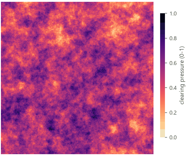
another date, on the same grid and coded the same way. We do not have a second date of this forest, so we make one:
a smooth random field of "clearing pressure" decides where the forest is cleared, which lets you run everything on
this page as it is. With your own maps, replace the two first nodes by two raster.read nodes.
In the application, two templates start these models: Templates > Connectivity > Network of a forest (MSPA) (MSPA, the components and the importance on a forest drawn by chance), and Templates > Patterns (GuidosToolbox) > Forest gain and loss (two dates, simple and morphological change, and the change of FAD).
The network of cores and bridges#
Model file (TOML)
format = "terraflux/1"

[[nodes]]
id = "forest"
op = "raster.read"
params = { path = "input.tif" }
note = "0 missing, 1 background, 2 forest."

[[nodes]]
id = "mspa"
op = "landscape.mspa"
inputs = { map = "forest.raster" }
params = { edge_width = 2 }
note = "Cores (the nodes) and bridges (the links)."

[[nodes]]
id = "components"
op = "networks.gtn_components"
inputs = { map = "mspa.map" }
note = "The networks, ECA and coherence."

[[nodes]]
id = "importance"
op = "networks.gtn_importance"
inputs = { map = "mspa.map" }
note = "dPC of every link and stepping stone."

[[nodes]]
id = "conefor"
op = "networks.conefor"
inputs = { map = "mspa.map" }
note = "The network as Conefor's two files."
Node 2 is the MSPA of part 2. The three network nodes take its map (the MSPA classes), not the forest: drag from
the output map of node 2 to the input map of each. They read only two of MSPA's classes, the cores (17, and 117
inside openings) and the bridges (33 and its variants), so the edge width of node 2 decides the network: a wider
edge shrinks the cores and turns more of the forest into bridges, which changes both the nodes and the links.
- In the library, open Habitat networks and click networks.gtn_components; it appears on the canvas.
- Drag from the
mapport of the MSPA node to themapport of the new node. - Do the same for networks.gtn_importance and networks.conefor.
- Select a node and press Ctrl+Enter to run the model up to it; its tables show in the Viewer.
The components#
networks.gtn_components groups the cores and bridges into 8-connected components and paints them: each network
in a colour of its own, isolated cores apart.

Its summary table:
| Value | |
|---|---|
| Components | 112 |
| Networks (with a bridge) | 49 |
| Isolated cores | 63 |
| Nodes (cores) | 420 |
| Links (bridges) | 258 |
| ECA (cells) | 155,517 |
| ECA_max (cells): all the core | 264,641 |
| Coherence | 58.8% |
How to read it: the forest has 264,641 cells of core. If they were all one network, a species moving along the
bridges could reach all of it, and ECA would be 264,641. They are split into 112 components, and the network is
worth a single block of 155,517 cells: 58.8% of the most it could be. Most of that comes from the large southern
network: because ECA squares the areas, one large network outweighs many small ones. The stats table lists every
component with its core and bridge cells, so you can find the largest networks and the cores left alone.
ECA is in cells because this map has no projected cell size; on a projected map (metres), it is also given in
hectares, and pixel_size sets the cell's size when the map does not carry it.
The importance of every link and stepping stone#
networks.gtn_importance removes every bridge in turn, and every stepping-stone core (a core with two links or
more), and measures how much the numerator of PC drops: its dPC. Its map paints, in GuidosToolbox's colours, the
links (reds) and the nodes (greens) whose dPC is within 1, 5 and 10% of the most important one's (at least 99, 95
and 90% of it). These classes are relative to the largest dPC, not the top 1, 5 and 10% of the links by number:
when one link is far more important than all the others, it may be the only one painted.


The links and nodes tables rank them:
| Link | Cells | Cores it touches | dPC (%) | Relative importance |
|---|---|---|---|---|
| 161 | 1,152 | 9 | 23.1 | 100 |
| 138 | 601 | 2 | 19.8 | 86 |
| 123 | 84 | 2 | 18.7 | 81 |
| 105 | 144 | 2 | 4.0 | 17 |
| 143 | 125 | 2 | 2.6 | 11 |
| Stepping stone | Cells | Links (degree) | dPC (%) | Relative importance |
|---|---|---|---|---|
| 304 | 101 | 10 | 19.8 | 100 |
| 366 | 20,690 | 32 | 19.7 | 99 |
| 230 | 1,197 | 2 | 18.5 | 93 |
| 176 | 12,933 | 5 | 4.4 | 22 |
| 257 | 3 | 2 | 2.6 | 13 |
Three things stand out, and they are why this analysis is worth running:
- Importance is very unequal. Of 258 links, three carry a dPC near 20% each; the fourth has 4%; the rest less than 3%. A handful of corridors hold the network together.
- A short link can matter as much as a long one. Link 123 is 84 cells, link 161 more than 1,100; their dPC is nearly the same, because what counts is what each one joins, not its length.
- A small core can be a key stepping stone. Node 304 is a core of 101 cells, less than a two-hundredth of node 366, but with ten links it is a hub: without it the network loses as much as without the largest core. Saura & Rubio (2010) call this the connector fraction of a patch's importance; such small cores are easy to overlook in a plan that ranks patches by area.
All of the top links are in component 62, the large southern network. That is a property of dPC: a link's importance is measured on the whole map's connectivity, so links inside small networks can never score high. Read the ranking as "where a loss would cost the region the most", not "the best link of every network".
In the literature
Saura et al. (2011b) combined MSPA's bridges with Conefor's importance indices in forests of central Spain and found that the structural connectors that matter most are a small share of the forest, and often not where a ranking by area would point. GuidosToolbox's GTN is the same idea, computed on the MSPA map itself.
The network in Conefor#
networks.conefor writes the network in the two files of Conefor (Saura & Torné, 2009): the cores as nodes with
their area (negative ids), the bridges as nodes of area 0 (positive ids), and a link of distance 1 from every bridge
to every core it touches. Here, 678 nodes (420 cores and 258 bridges) and 625 links. Save nodes_txt and
links_txt from the Node pane, or make them outputs of a model run from the command line, to compute the other
indices of Conefor (IIC, the fractions of dPC); the habitat networks tutorials do
those inside Terraflux, on distances between patches rather than on the bridges.
Change between two dates#
The second date#
Model file (TOML)
format = "terraflux/1"

[[nodes]]
id = "before"
op = "raster.read"
params = { path = "input.tif" }
note = "Date A."

[[nodes]]
id = "pressure"
op = "nlm.gaussian_field"
params = { rows = 1000, columns = 1000, range = 60, seed = 28 }
note = "Where clearing presses, 0 to 1."

[[nodes]]
id = "after"
op = "raster.calc"
inputs = { f = "before.raster", p = "pressure.map" }
params = { expression = "1 if f == 2 and p > 0.8 else 1 if f == 2 and p > 0.55 and nbsum(f == 1, 3) >= 1 else 2 if f == 1 and p < 0.15 and nbsum(f == 2, 1) >= 4 else f" }
note = "Date B: cleared where pressed (with your maps: a raster.read)."

[[nodes]]
id = "simple"
op = "change.simple"
inputs = { before = "before.raster", after = "after.map" }

[[nodes]]
id = "morphological"
op = "change.morphological"
inputs = { before = "before.raster", after = "after.map" }

[[nodes]]
id = "mspa_a"
op = "landscape.mspa"
inputs = { map = "before.raster" }
params = { edge_width = 2 }

[[nodes]]
id = "mspa_b"
op = "landscape.mspa"
inputs = { map = "after.map" }
params = { edge_width = 2 }

[[nodes]]
id = "network_b"
op = "networks.gtn_components"
inputs = { map = "mspa_b.map" }
Nodes 2 and 3 only make a second date to work with. nlm.gaussian_field draws a smooth surface from 0 to 1 whose
patches are about 60 cells across; raster.calc then clears the forest (2 becomes 1) everywhere the pressure is
above 0.8, eats the forest's edges where it is above 0.55 (the forest cells with at least one background cell within
3 cells: nbsum(f == 1, 3) >= 1 counts the background cells of the 7 × 7 window, since f == 1 is 1 on them and 0
elsewhere), and lets a little forest regrow where it is below 0.15, in background cells with at least 4 forest cells
around them. It is a
caricature of selective clearing, but it does two things real change does: whole blocks go, and edges retreat.


The forest goes from 428,490 cells to 354,172: a net loss of 74,318 cells, 17.3% of the forest.
Simple change#
change.simple compares the two maps cell by cell, in GuidosToolbox's codes: 11 stable background, 12 gain, 21
loss, 22 stable forest, 255 missing at either date. Both inputs are maps of the same grid; connect the date A map to
before and the date B map to after (swapping them swaps gain and loss).

Its stats table: 354,098 cells of stable forest, 74,392 of loss, 74 of gain, 571,166 of stable background and 270
missing. The loss is 17.4% of the forest of date A. This is the right number for "how much forest was lost"
if the two maps are perfectly comparable.
Morphological change#
change.morphological takes the same two inputs and gives the same codes plus 176, spurious change.


Its stats table:
| Cells | |
|---|---|
| Forest at date A | 428,490 |
| Forest at date B | 354,172 |
| Net change | −74,318 |
| Structural loss | 45,552 |
| Structural gain | 0 |
| Spurious change | 36,187 |
| Stable forest | 351,200 |
| Stable background | 566,791 |
| Elasticity | 1.23 |
How to read it:
- Almost half of the changed cells are spurious. Of the 74,466 cells that changed (loss and gain), 36,187 are thin strips along the edges, not connected to any change deep in a forest or a field. Here we know they are real: node 3 ate the edges on purpose, up to 3 cells deep. With two maps from different sources they would be mostly noise, and that is the point: MCD cannot tell a real retreat of the edge by a cell or two from a misregistration. It reports the change that a shift of the maps could not have made.
- The structural loss is not the area cleared. Its 45,552 cells are 38,279 of the cells cleared, plus 2,898 that were forest at both dates and 4,375 that were background at both: MCD closes the areas of loss (a morphological closing of 3 × 3 cells), which fills small islands and gaps inside a clearing. The map shows where the forest's structure was lost; for the area cleared, use simple change.
- The 74 cells of gain are all spurious: regrowth in small gaps never reaches the interior of a field.
- Elasticity 1.23: the interior of the forest shrank 1.23 times faster than the forest, about 21% against 17%. Both kinds of loss are here: the blocks cleared pierced the interior, and the edges that retreated took mostly forest that was not interior, which keeps the elasticity near 1.
MSPA and the network at both dates#
The same MSPA on both dates (nodes 6 and 7) shows how the forest's structure changed, beyond how much.


Where did the forest of date A go? Following every cell from its class at A to its class at B:
| Class at A | Cells | Still the same class | Became a bridge | Lost (background) |
|---|---|---|---|---|
| Core | 264,641 | 77.1% | 3.2% | 6.2% |
| Edge | 59,657 | 44.7% | 6.8% | 33.4% |
| Bridge | 27,772 | 44.5% | 40.9% | |
| Loop | 20,237 | 45.6% | 8.4% | 37.0% |
| Branch | 20,535 | 48.0% | 1.5% | 34.4% |
| Islet | 26,040 | 67.1% | 0.0% | 32.9% |
| Perforation | 9,608 | 29.6% | 4.6% | 38.2% |
(The full table, with every class at B, is in mspa-transitions.csv.)
Two lessons. A loss of 17% of the forest cost it 23% of its core (264,641 cells at A, 57.6% of 354,172 = about 204,000 at B), although only 6.2% of the core was cleared: the rest became edge, loops and bridges as the clearings came closer. And the bridges, a small share of the forest, were lost at the highest rate, 40.9%, since they are the narrowest forest and an edge that retreats by 3 cells swallows them. A few bridges cleared can cut a network in pieces; the network at both dates shows it:
| Date A | Date B | |
|---|---|---|
| Components | 112 | 110 |
| Networks | 49 | 55 |
| Isolated cores | 63 | 55 |
| Nodes (cores) | 420 | 370 |
| Links (bridges) | 258 | 188 |
| ECA (cells) | 155,517 | 62,645 |
| ECA_max (cells) | 264,641 | 204,135 |
| Coherence | 58.8% | 30.7% |
The forest lost 17% of its area and 23% of its core, but 60% of its equivalent connected area: its links fell from 258 to 188, the large southern network broke into pieces, and the coherence fell by half. This is why reports of change should give a measure of connectivity beside the area: the area alone hides most of the damage.
Report it
For a change between two dates, report: the forest at both dates and the net change; the simple gain and loss (and the share of the morphological change that is spurious, as a check of how comparable the maps are); MSPA's shares at both dates with the same edge width; and ECA and the coherence at both dates. A figure of the morphological change and a pair of MSPA maps of a zoom show where it happened.
MSPA of large maps#
landscape.mspa_tiled takes the map as rasters on disk (the output raster of raster.read, not map), reads
and runs it tile by tile, and writes the result to a GeoTIFF (path). Two settings decide the tiles:
tile_size: a tile's side in cells, its overlap included (default 6,500);overlap: how many cells two neighbouring tiles share (default 2,000).
Memory grows with the tile's area, not the map's. The other settings are MSPA's own, and must be the same as in an MSPA of the whole map you would compare it with.
A national map takes a while. In the application, the node tells which tile it is on (tiled: tile 4 of 16 in the
status bar, and a bar along the bottom of its box that fills as the tiles are done), and Stop stops it between
two tiles: the tile being computed is finished, the others are not started. landscape.mspa of a whole map cannot
stop in the middle; after Stop it goes on in the background until it is done.
Model file (TOML)
format = "terraflux/1"

[[nodes]]
id = "forest"
op = "raster.read"
params = { path = "input.tif" }

[[nodes]]
id = "tiled"
op = "landscape.mspa_tiled"
inputs = { map = "forest.raster" }
params = { edge_width = 2, tile_size = 300, overlap = 60, path = "mspa_tiled.tif" }
note = "Written to disk, tile by tile."

[[nodes]]
id = "whole"
op = "landscape.mspa"
inputs = { map = "forest.raster" }
params = { edge_width = 2 }
note = "For comparison."
To see how far the approximation goes, we ran it with tiles of 300 cells (a tiny tile, to make the seams many) and an overlap of 20 and of 60 cells, and compared both with MSPA of the whole map.


With an overlap of 20 cells, 1,312 forest cells (0.3% of the forest) get another class than in MSPA of the whole map: mostly bridges and branches whose ends lie in another tile, whose role is decided by cores the tile does not see. An overlap of 60 halves that, to 700. The orange areas are the other kind of error: a large clearing inside a forest that spans several tiles is not recognised as enclosed (a core-opening) because no tile holds the whole forest around it. That error does not shrink with a larger overlap here, because the forest around those clearings is hundreds of cells across: only an overlap larger than the objects removes it.
The rule of thumb: the overlap should be larger than the largest object whose structure matters, or at least larger than the longest bridges. GuidosToolbox's defaults (tiles of 6,500 cells and an overlap of 2,000) suit national maps at 30 m; with them, maps of a few billion cells run in a few gigabytes of memory.
Larger than memory, in general
Rasters on disk flow through Terraflux without being loaded when the operators read them in blocks; MSPA cannot (a cell's class depends on the whole object), which is why it has a tiled variant. The large data tutorials cover the other ways: blocks, windows, batches over many files.
Settings that change the answer#
- The edge width of the MSPA that feeds the network. A wider edge makes smaller cores and more bridges, so more nodes and links, and a lower ECA. Choose it as in part 2, from the depth of edge effects for the species, and keep it the same at both dates.
- The connectivity (8 by default). With 4 neighbours, bridges that hang by a corner break, and networks split. GTN groups its components with 8 neighbours; run MSPA with the same.
- The comparability of the two dates. The share of spurious change is a diagnostic: when it is large on maps that should differ little, they were made differently or are shifted.
- The overlap of the tiled MSPA, as above.
Common pitfalls#
- Comparing a network across maps of different cell sizes. Bridges and cores depend on the resolution (a strip of trees 20 m wide is a bridge at 10 m and nothing at 30 m). Compare networks only on maps of the same resolution and minimum mapping unit.
- Reading ECA in cells as hectares. On a map in degrees (like this sample) ECA is in cells; project the map to an
equal-area system first, or give
pixel_size. - Taking dPC as the importance for every species. It is structural: it assumes a species moves along the forest's bridges and nowhere else. A species that crosses fields needs a functional network (habitat networks).
- Reporting MCD's loss as the area cleared. The morphological loss includes the stable cells filled in by its closing and leaves out the thin strips; report the area from simple change.
- Swapping the dates.
beforeis the first date; with the maps swapped, loss becomes gain. - Two dates on different grids. Both maps must have the same rows, columns and cells; reproject and resample one onto the other first (one grid).
Going further#
- Fragmentation: the forest's density around every cell at many scales, and its change
between dates (
change.fad,change.fos). - Habitat networks: Conefor's connectivity indices on distances between patches, ProtConn and the importance of each patch for a species with a dispersal distance.
- Change detection: transition matrices and intensity analysis for maps of many classes.
- The operator reference:
networks.gtn_components,networks.gtn_importance,networks.conefor,change.simple,change.morphological,landscape.mspa_tiled.
References#
- Riitters, K. H., & Wickham, J. D. (2012). Decline of forest interior conditions in the conterminous United States. Scientific Reports, 2, 653. https://doi.org/10.1038/srep00653
- Saura, S., Estreguil, C., Mouton, C., & Rodríguez-Freire, M. (2011a). Network analysis to assess landscape connectivity trends: application to European forests (1990–2000). Ecological Indicators, 11(2), 407–416. https://doi.org/10.1016/j.ecolind.2010.06.011
- Saura, S., & Pascual-Hortal, L. (2007). A new habitat availability index to integrate connectivity in landscape conservation planning: comparison with existing indices and application to a case study. Landscape and Urban Planning, 83(2–3), 91–103. https://doi.org/10.1016/j.landurbplan.2007.03.005
- Saura, S., & Rubio, L. (2010). A common currency for the different ways in which patches and links can contribute to habitat availability and connectivity in the landscape. Ecography, 33(3), 523–537. https://doi.org/10.1111/j.1600-0587.2009.05760.x
- Saura, S., & Torné, J. (2009). Conefor Sensinode 2.2: a software package for quantifying the importance of habitat patches for landscape connectivity. Environmental Modelling & Software, 24(1), 135–139. https://doi.org/10.1016/j.envsoft.2008.05.005
- Saura, S., Vogt, P., Velázquez, J., Hernando, A., & Tejera, R. (2011b). Key structural forest connectors can be identified by combining landscape spatial pattern and network analyses. Forest Ecology and Management, 262(2), 150–160. https://doi.org/10.1016/j.foreco.2011.03.017
- Vogt, P., Ferrari, J. R., Lookingbill, T. R., Gardner, R. H., Riitters, K. H., & Ostapowicz, K. (2009). Mapping functional connectivity. Ecological Indicators, 9(1), 64–71. https://doi.org/10.1016/j.ecolind.2008.01.011
- Vogt, P., & Riitters, K. (2017). GuidosToolbox: universal digital image object analysis. European Journal of Remote Sensing, 50(1), 352–361. https://doi.org/10.1080/22797254.2017.1330650
- Wickham, J. D., Riitters, K. H., Wade, T. G., & Homer, C. (2008). Temporal change in fragmentation of continental US forests. Landscape Ecology. https://doi.org/10.1007/s10980-008-9258-z